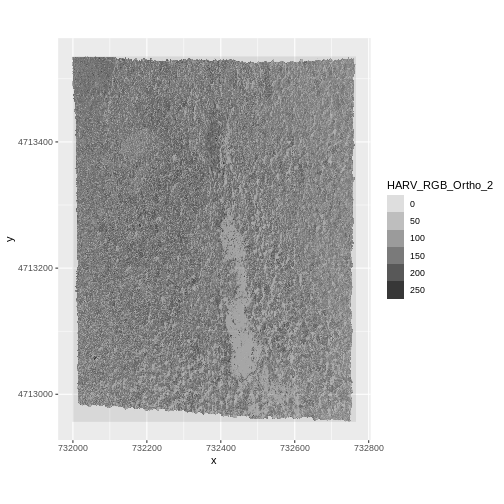
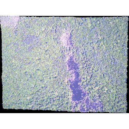
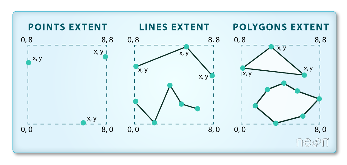
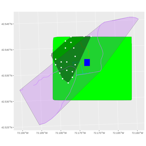
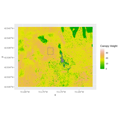
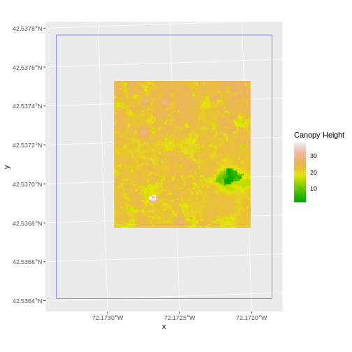
Image 1 of 1: ‘Extent image’
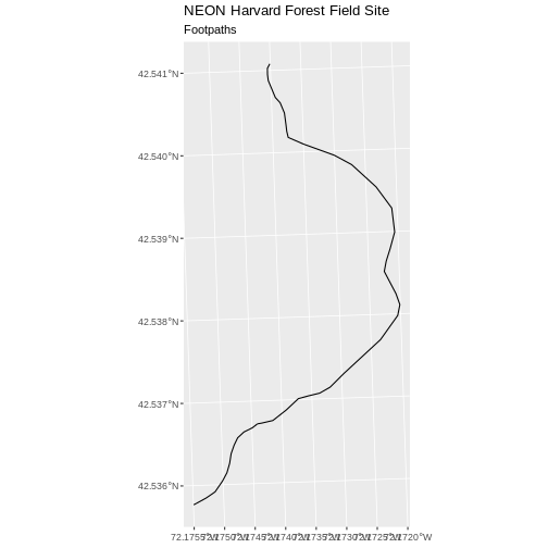
Image 1 of 1: ‘Map of the footpaths in the study area.’
Map of the footpaths in the study area.
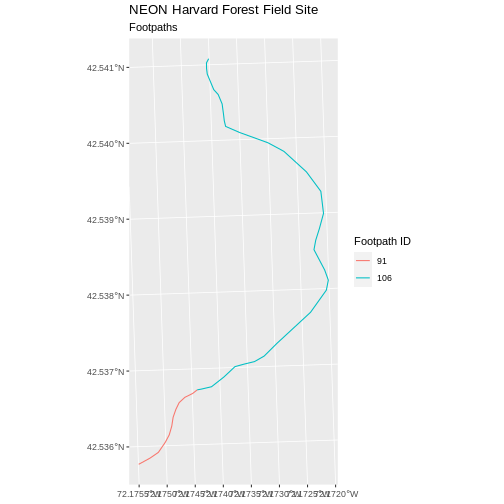
Image 1 of 1: ‘Map of the footpaths in the study area where each feature is colored differently.’
Map of the footpaths in the study area where each feature is colored
differently.
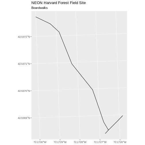
Image 1 of 1: ‘Map of the boardwalks in the study area.’
Map of the boardwalks in the study area.
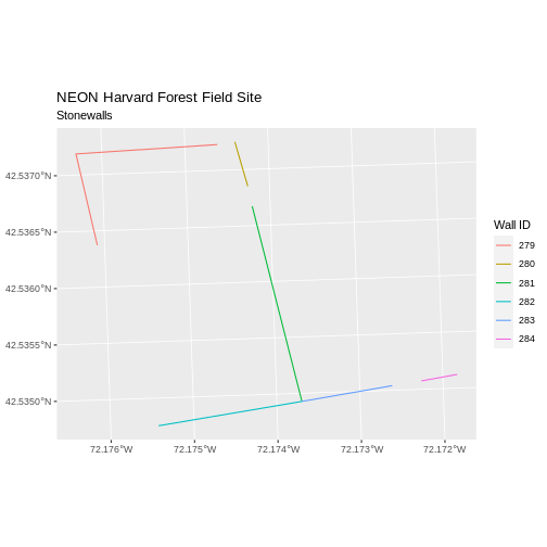
Image 1 of 1: ‘Map of the stone walls in the study area where each feature is colored differently.’
Map of the stone walls in the study area where each feature is colored
differently.
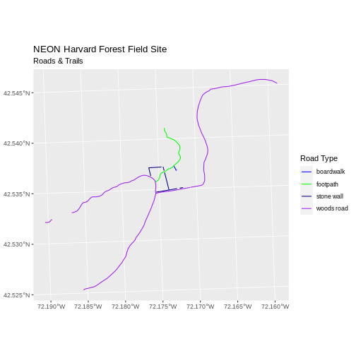
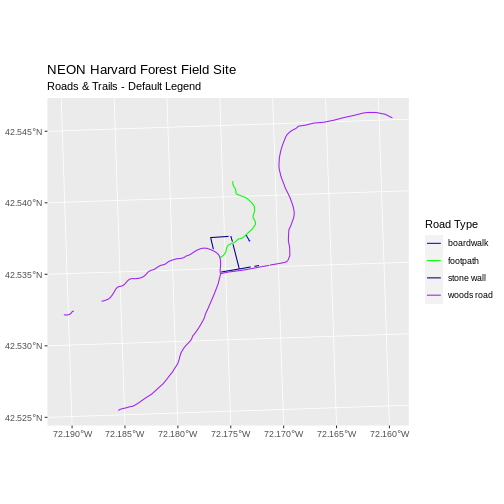
Image 1 of 1: ‘Roads and trails in the area.’
Roads and trails in the area.
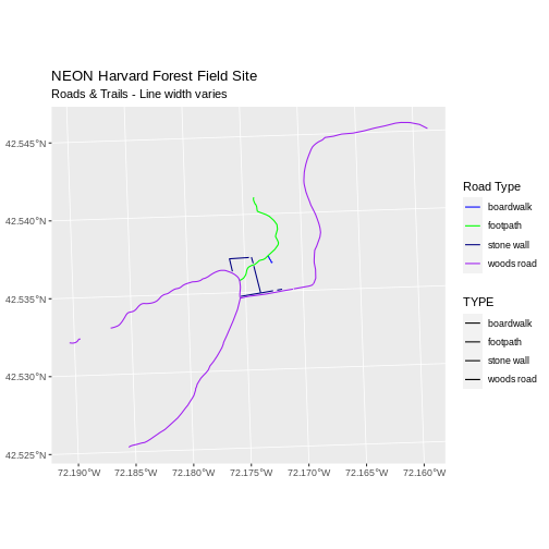
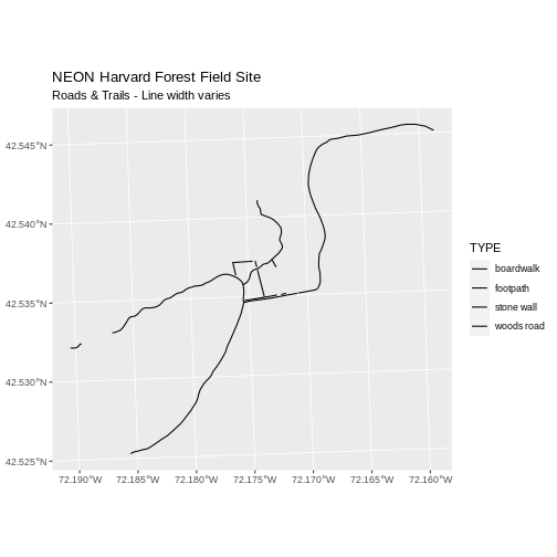
Image 1 of 1: ‘Roads and trails in the area demonstrating how to use different line thickness and colors.’
Roads and trails in the area demonstrating how to use different line
thickness and colors.
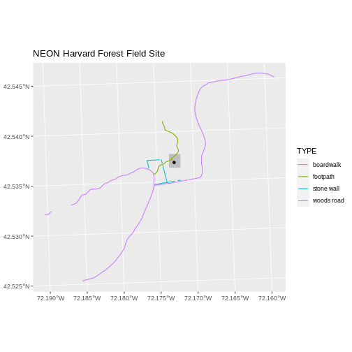
Image 1 of 1: ‘Roads and trails in the area with different line thickness for each type of paths.’
Roads and trails in the area with different line thickness for each type
of paths.
Image 1 of 1: ‘Roads and trails in the study area using thicker lines than the previous figure.’
Roads and trails in the study area using thicker lines than the previous
figure.
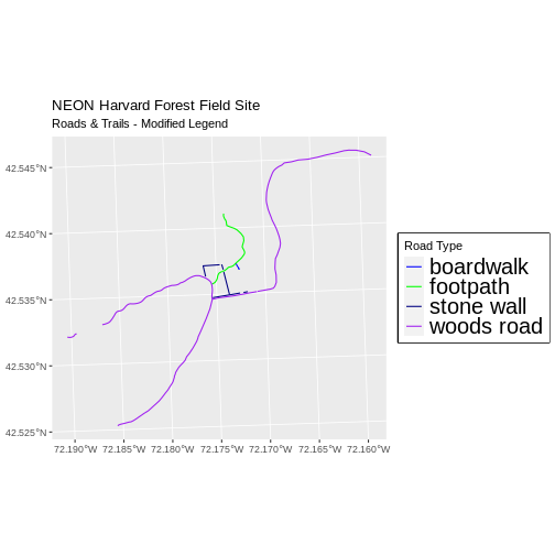
Image 1 of 1: ‘Map of the paths in the study area with large-font and border around the legend.’
Map of the paths in the study area with large-font and border around the
legend.
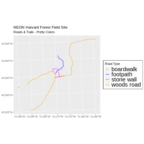
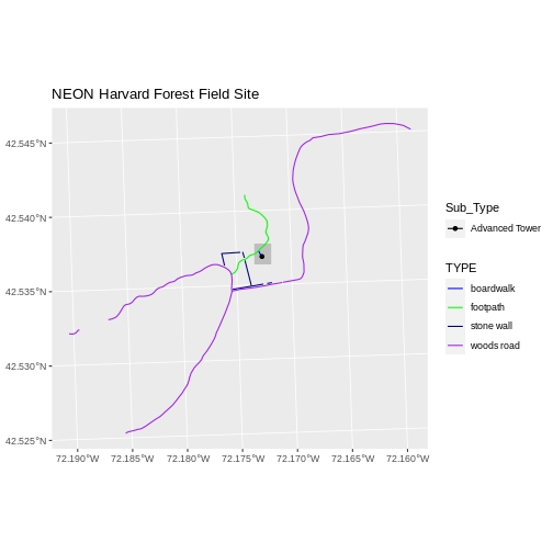
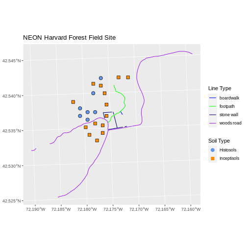
Image 1 of 1: ‘Map of the paths in the study area using a different color palette.’
Map of the paths in the study area using a different color palette.
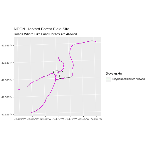
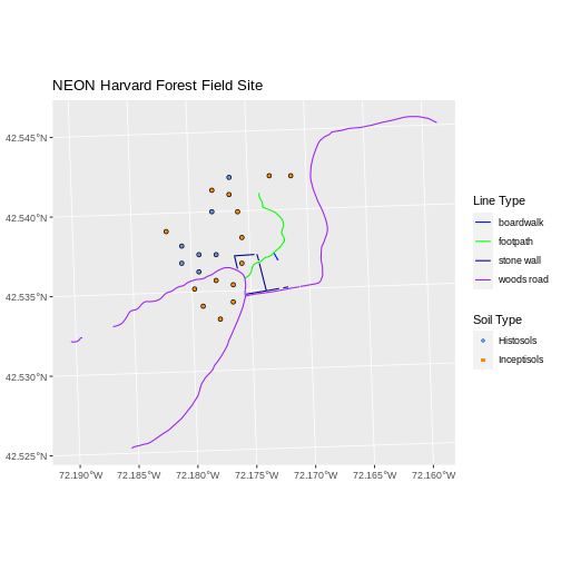
Image 1 of 1: ‘Roads and trails in the area highlighting paths where horses and bikes are allowed.’
Roads and trails in the area highlighting paths where horses and bikes
are allowed.
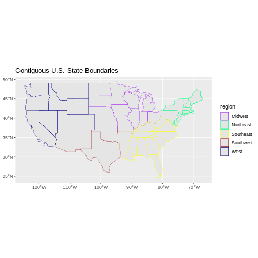
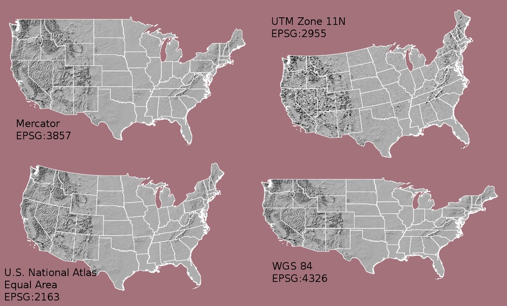
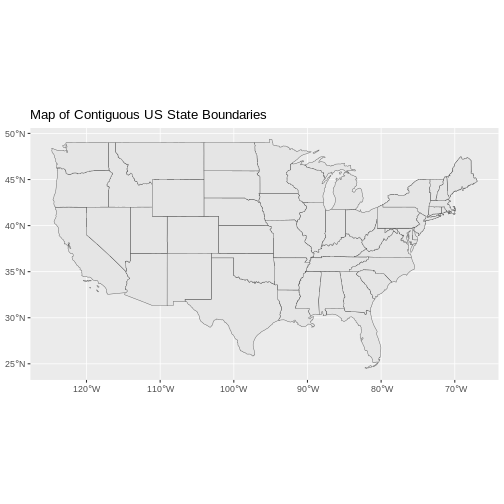
Image 1 of 1: ‘Map of the continental United States where the state lines are colored by region.’
Map of the continental United States where the state lines are colored
by region.


