Content from Introduction and setup
Last updated on 2023-03-14 | Edit this page
Overview
Questions
Objectives
- Install required packages.
- Download the data.
Download data
The data we will use in this lesson is obtained from the Gene Expression Omnibus, accession number GSE96870.
R
dir.create("data", showWarnings = FALSE)
download.file(
    url = "https://github.com/Bioconductor/bioconductor-teaching/blob/master/data/GSE96870/GSE96870_counts_cerebellum.csv?raw=true",
    destfile = "data/GSE96870_counts_cerebellum.csv"
)

download.file(
    url = "https://github.com/Bioconductor/bioconductor-teaching/blob/master/data/GSE96870/GSE96870_coldata_cerebellum.csv?raw=true",
    destfile = "data/GSE96870_coldata_cerebellum.csv"
)

download.file(
    url = "https://github.com/Bioconductor/bioconductor-teaching/blob/master/data/GSE96870/GSE96870_coldata_all.csv?raw=true",
    destfile = "data/GSE96870_coldata_all.csv"
)

download.file(
    url = "https://github.com/Bioconductor/bioconductor-teaching/blob/master/data/GSE96870/GSE96870_rowranges.tsv?raw=true",
    destfile = "data/GSE96870_rowranges.tsv"
)
Content from Introduction to RNA-seq
Last updated on 2023-03-14 | Edit this page
Overview
Questions
- What is RNA-seq?
Objectives
- Explain what RNA-seq is and what the generated data looks like.
- Provide an overview of common quality control steps for the raw data.
- Explain how gene expression levels can be estimated from raw data.
Content from Experimental design
Last updated on 2023-03-14 | Edit this page
Overview
Questions
- How do we design experiments optimally?
- How do we interpret a given design?
Objectives
- Explain the formula notation and design matrices.
- Explore different designs and learn how to interpret coefficients.
R
suppressPackageStartupMessages({
    library(SummarizedExperiment)
    library(ExploreModelMatrix)
    library(dplyr)
})
R
meta <- read.csv("data/GSE96870_coldata_all.csv", row.names = 1)
meta
OUTPUT
                     title geo_accession     organism     age    sex
GSM2545336 CNS_RNA-seq_10C    GSM2545336 Mus musculus 8 weeks Female
GSM2545337 CNS_RNA-seq_11C    GSM2545337 Mus musculus 8 weeks Female
GSM2545338 CNS_RNA-seq_12C    GSM2545338 Mus musculus 8 weeks Female
GSM2545339 CNS_RNA-seq_13C    GSM2545339 Mus musculus 8 weeks Female
GSM2545340 CNS_RNA-seq_14C    GSM2545340 Mus musculus 8 weeks   Male
GSM2545341 CNS_RNA-seq_17C    GSM2545341 Mus musculus 8 weeks   Male
GSM2545342  CNS_RNA-seq_1C    GSM2545342 Mus musculus 8 weeks Female
GSM2545343 CNS_RNA-seq_20C    GSM2545343 Mus musculus 8 weeks   Male
GSM2545344 CNS_RNA-seq_21C    GSM2545344 Mus musculus 8 weeks Female
GSM2545345 CNS_RNA-seq_22C    GSM2545345 Mus musculus 8 weeks   Male
GSM2545346 CNS_RNA-seq_25C    GSM2545346 Mus musculus 8 weeks   Male
GSM2545347 CNS_RNA-seq_26C    GSM2545347 Mus musculus 8 weeks   Male
GSM2545348 CNS_RNA-seq_27C    GSM2545348 Mus musculus 8 weeks Female
GSM2545349 CNS_RNA-seq_28C    GSM2545349 Mus musculus 8 weeks   Male
GSM2545350 CNS_RNA-seq_29C    GSM2545350 Mus musculus 8 weeks   Male
GSM2545351  CNS_RNA-seq_2C    GSM2545351 Mus musculus 8 weeks Female
GSM2545352 CNS_RNA-seq_30C    GSM2545352 Mus musculus 8 weeks Female
GSM2545353  CNS_RNA-seq_3C    GSM2545353 Mus musculus 8 weeks Female
GSM2545354  CNS_RNA-seq_4C    GSM2545354 Mus musculus 8 weeks   Male
GSM2545355 CNS_RNA-seq_571    GSM2545355 Mus musculus 8 weeks   Male
GSM2545356 CNS_RNA-seq_574    GSM2545356 Mus musculus 8 weeks   Male
GSM2545357 CNS_RNA-seq_575    GSM2545357 Mus musculus 8 weeks   Male
GSM2545358 CNS_RNA-seq_583    GSM2545358 Mus musculus 8 weeks Female
GSM2545359 CNS_RNA-seq_585    GSM2545359 Mus musculus 8 weeks Female
GSM2545360 CNS_RNA-seq_589    GSM2545360 Mus musculus 8 weeks   Male
GSM2545361 CNS_RNA-seq_590    GSM2545361 Mus musculus 8 weeks   Male
GSM2545362  CNS_RNA-seq_5C    GSM2545362 Mus musculus 8 weeks Female
GSM2545363  CNS_RNA-seq_6C    GSM2545363 Mus musculus 8 weeks   Male
GSM2545364 CNS_RNA-seq_709    GSM2545364 Mus musculus 8 weeks Female
GSM2545365 CNS_RNA-seq_710    GSM2545365 Mus musculus 8 weeks Female
GSM2545366 CNS_RNA-seq_711    GSM2545366 Mus musculus 8 weeks Female
GSM2545367 CNS_RNA-seq_713    GSM2545367 Mus musculus 8 weeks   Male
GSM2545368 CNS_RNA-seq_728    GSM2545368 Mus musculus 8 weeks   Male
GSM2545369 CNS_RNA-seq_729    GSM2545369 Mus musculus 8 weeks   Male
GSM2545370 CNS_RNA-seq_730    GSM2545370 Mus musculus 8 weeks Female
GSM2545371 CNS_RNA-seq_731    GSM2545371 Mus musculus 8 weeks Female
GSM2545372 CNS_RNA-seq_733    GSM2545372 Mus musculus 8 weeks   Male
GSM2545373 CNS_RNA-seq_735    GSM2545373 Mus musculus 8 weeks   Male
GSM2545374 CNS_RNA-seq_736    GSM2545374 Mus musculus 8 weeks Female
GSM2545375 CNS_RNA-seq_738    GSM2545375 Mus musculus 8 weeks Female
GSM2545376 CNS_RNA-seq_740    GSM2545376 Mus musculus 8 weeks Female
GSM2545377 CNS_RNA-seq_741    GSM2545377 Mus musculus 8 weeks Female
GSM2545378 CNS_RNA-seq_742    GSM2545378 Mus musculus 8 weeks   Male
GSM2545379 CNS_RNA-seq_743    GSM2545379 Mus musculus 8 weeks   Male
GSM2545380  CNS_RNA-seq_9C    GSM2545380 Mus musculus 8 weeks Female
             infection  strain time     tissue mouse
GSM2545336  InfluenzaA C57BL/6 Day8 Cerebellum    14
GSM2545337 NonInfected C57BL/6 Day0 Cerebellum     9
GSM2545338 NonInfected C57BL/6 Day0 Cerebellum    10
GSM2545339  InfluenzaA C57BL/6 Day4 Cerebellum    15
GSM2545340  InfluenzaA C57BL/6 Day4 Cerebellum    18
GSM2545341  InfluenzaA C57BL/6 Day8 Cerebellum     6
GSM2545342  InfluenzaA C57BL/6 Day8 Cerebellum     5
GSM2545343 NonInfected C57BL/6 Day0 Cerebellum    11
GSM2545344  InfluenzaA C57BL/6 Day4 Cerebellum    22
GSM2545345  InfluenzaA C57BL/6 Day4 Cerebellum    13
GSM2545346  InfluenzaA C57BL/6 Day8 Cerebellum    23
GSM2545347  InfluenzaA C57BL/6 Day8 Cerebellum    24
GSM2545348 NonInfected C57BL/6 Day0 Cerebellum     8
GSM2545349 NonInfected C57BL/6 Day0 Cerebellum     7
GSM2545350  InfluenzaA C57BL/6 Day4 Cerebellum     1
GSM2545351  InfluenzaA C57BL/6 Day8 Cerebellum    16
GSM2545352  InfluenzaA C57BL/6 Day4 Cerebellum    21
GSM2545353 NonInfected C57BL/6 Day0 Cerebellum     4
GSM2545354 NonInfected C57BL/6 Day0 Cerebellum     2
GSM2545355  InfluenzaA C57BL/6 Day4 Spinalcord     1
GSM2545356 NonInfected C57BL/6 Day0 Spinalcord     2
GSM2545357 NonInfected C57BL/6 Day0 Spinalcord     3
GSM2545358 NonInfected C57BL/6 Day0 Spinalcord     4
GSM2545359  InfluenzaA C57BL/6 Day8 Spinalcord     5
GSM2545360  InfluenzaA C57BL/6 Day8 Spinalcord     6
GSM2545361 NonInfected C57BL/6 Day0 Spinalcord     7
GSM2545362  InfluenzaA C57BL/6 Day4 Cerebellum    20
GSM2545363  InfluenzaA C57BL/6 Day4 Cerebellum    12
GSM2545364 NonInfected C57BL/6 Day0 Spinalcord     8
GSM2545365 NonInfected C57BL/6 Day0 Spinalcord     9
GSM2545366 NonInfected C57BL/6 Day0 Spinalcord    10
GSM2545367 NonInfected C57BL/6 Day0 Spinalcord    11
GSM2545368  InfluenzaA C57BL/6 Day4 Spinalcord    12
GSM2545369  InfluenzaA C57BL/6 Day4 Spinalcord    13
GSM2545370  InfluenzaA C57BL/6 Day8 Spinalcord    14
GSM2545371  InfluenzaA C57BL/6 Day4 Spinalcord    15
GSM2545372  InfluenzaA C57BL/6 Day8 Spinalcord    17
GSM2545373  InfluenzaA C57BL/6 Day4 Spinalcord    18
GSM2545374  InfluenzaA C57BL/6 Day8 Spinalcord    19
GSM2545375  InfluenzaA C57BL/6 Day4 Spinalcord    20
GSM2545376  InfluenzaA C57BL/6 Day4 Spinalcord    21
GSM2545377  InfluenzaA C57BL/6 Day4 Spinalcord    22
GSM2545378  InfluenzaA C57BL/6 Day8 Spinalcord    23
GSM2545379  InfluenzaA C57BL/6 Day8 Spinalcord    24
GSM2545380  InfluenzaA C57BL/6 Day8 Cerebellum    19
R
vd <- VisualizeDesign(sampleData = meta,
                      designFormula = ~ tissue + time + sex)
vd$cooccurrenceplots
OUTPUT
$`tissue = Cerebellum`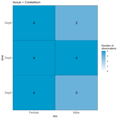
OUTPUT
$`tissue = Spinalcord`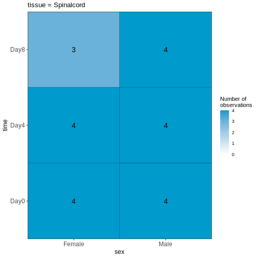
Compare males and females, non-infected spinal cord
R
meta_noninf_spc <- meta %>% filter(time == "Day0" &
                                       tissue == "Spinalcord")
meta_noninf_spc
OUTPUT
                     title geo_accession     organism     age    sex
GSM2545356 CNS_RNA-seq_574    GSM2545356 Mus musculus 8 weeks   Male
GSM2545357 CNS_RNA-seq_575    GSM2545357 Mus musculus 8 weeks   Male
GSM2545358 CNS_RNA-seq_583    GSM2545358 Mus musculus 8 weeks Female
GSM2545361 CNS_RNA-seq_590    GSM2545361 Mus musculus 8 weeks   Male
GSM2545364 CNS_RNA-seq_709    GSM2545364 Mus musculus 8 weeks Female
GSM2545365 CNS_RNA-seq_710    GSM2545365 Mus musculus 8 weeks Female
GSM2545366 CNS_RNA-seq_711    GSM2545366 Mus musculus 8 weeks Female
GSM2545367 CNS_RNA-seq_713    GSM2545367 Mus musculus 8 weeks   Male
             infection  strain time     tissue mouse
GSM2545356 NonInfected C57BL/6 Day0 Spinalcord     2
GSM2545357 NonInfected C57BL/6 Day0 Spinalcord     3
GSM2545358 NonInfected C57BL/6 Day0 Spinalcord     4
GSM2545361 NonInfected C57BL/6 Day0 Spinalcord     7
GSM2545364 NonInfected C57BL/6 Day0 Spinalcord     8
GSM2545365 NonInfected C57BL/6 Day0 Spinalcord     9
GSM2545366 NonInfected C57BL/6 Day0 Spinalcord    10
GSM2545367 NonInfected C57BL/6 Day0 Spinalcord    11
R
vd <- VisualizeDesign(sampleData = meta_noninf_spc,
                      designFormula = ~ sex)
vd$designmatrix
OUTPUT
           (Intercept) sexMale
GSM2545356           1       1
GSM2545357           1       1
GSM2545358           1       0
GSM2545361           1       1
GSM2545364           1       0
GSM2545365           1       0
GSM2545366           1       0
GSM2545367           1       1
R
vd$plotlist
OUTPUT
[[1]]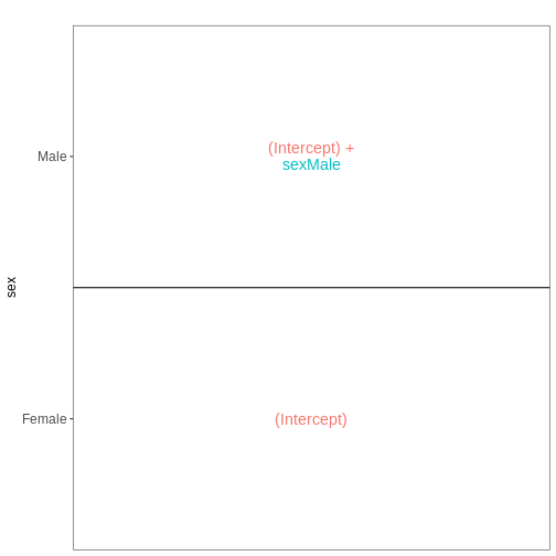
R
meta_male_spc <- meta %>% filter(sex == "Male" & tissue == "Spinalcord")
meta_male_spc
OUTPUT
                     title geo_accession     organism     age  sex   infection
GSM2545355 CNS_RNA-seq_571    GSM2545355 Mus musculus 8 weeks Male  InfluenzaA
GSM2545356 CNS_RNA-seq_574    GSM2545356 Mus musculus 8 weeks Male NonInfected
GSM2545357 CNS_RNA-seq_575    GSM2545357 Mus musculus 8 weeks Male NonInfected
GSM2545360 CNS_RNA-seq_589    GSM2545360 Mus musculus 8 weeks Male  InfluenzaA
GSM2545361 CNS_RNA-seq_590    GSM2545361 Mus musculus 8 weeks Male NonInfected
GSM2545367 CNS_RNA-seq_713    GSM2545367 Mus musculus 8 weeks Male NonInfected
GSM2545368 CNS_RNA-seq_728    GSM2545368 Mus musculus 8 weeks Male  InfluenzaA
GSM2545369 CNS_RNA-seq_729    GSM2545369 Mus musculus 8 weeks Male  InfluenzaA
GSM2545372 CNS_RNA-seq_733    GSM2545372 Mus musculus 8 weeks Male  InfluenzaA
GSM2545373 CNS_RNA-seq_735    GSM2545373 Mus musculus 8 weeks Male  InfluenzaA
GSM2545378 CNS_RNA-seq_742    GSM2545378 Mus musculus 8 weeks Male  InfluenzaA
GSM2545379 CNS_RNA-seq_743    GSM2545379 Mus musculus 8 weeks Male  InfluenzaA
            strain time     tissue mouse
GSM2545355 C57BL/6 Day4 Spinalcord     1
GSM2545356 C57BL/6 Day0 Spinalcord     2
GSM2545357 C57BL/6 Day0 Spinalcord     3
GSM2545360 C57BL/6 Day8 Spinalcord     6
GSM2545361 C57BL/6 Day0 Spinalcord     7
GSM2545367 C57BL/6 Day0 Spinalcord    11
GSM2545368 C57BL/6 Day4 Spinalcord    12
GSM2545369 C57BL/6 Day4 Spinalcord    13
GSM2545372 C57BL/6 Day8 Spinalcord    17
GSM2545373 C57BL/6 Day4 Spinalcord    18
GSM2545378 C57BL/6 Day8 Spinalcord    23
GSM2545379 C57BL/6 Day8 Spinalcord    24
R
vd <- VisualizeDesign(sampleData = meta_male_spc, designFormula = ~ time)
vd$designmatrix
OUTPUT
           (Intercept) timeDay4 timeDay8
GSM2545355           1        1        0
GSM2545356           1        0        0
GSM2545357           1        0        0
GSM2545360           1        0        1
GSM2545361           1        0        0
GSM2545367           1        0        0
GSM2545368           1        1        0
GSM2545369           1        1        0
GSM2545372           1        0        1
GSM2545373           1        1        0
GSM2545378           1        0        1
GSM2545379           1        0        1
R
vd$plotlist
OUTPUT
[[1]]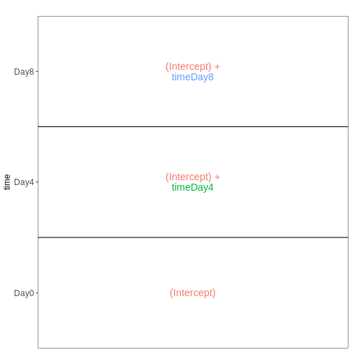
Factorial design without interactions
R
meta_noninf <- meta %>% filter(time == "Day0")
meta_noninf
OUTPUT
                     title geo_accession     organism     age    sex
GSM2545337 CNS_RNA-seq_11C    GSM2545337 Mus musculus 8 weeks Female
GSM2545338 CNS_RNA-seq_12C    GSM2545338 Mus musculus 8 weeks Female
GSM2545343 CNS_RNA-seq_20C    GSM2545343 Mus musculus 8 weeks   Male
GSM2545348 CNS_RNA-seq_27C    GSM2545348 Mus musculus 8 weeks Female
GSM2545349 CNS_RNA-seq_28C    GSM2545349 Mus musculus 8 weeks   Male
GSM2545353  CNS_RNA-seq_3C    GSM2545353 Mus musculus 8 weeks Female
GSM2545354  CNS_RNA-seq_4C    GSM2545354 Mus musculus 8 weeks   Male
GSM2545356 CNS_RNA-seq_574    GSM2545356 Mus musculus 8 weeks   Male
GSM2545357 CNS_RNA-seq_575    GSM2545357 Mus musculus 8 weeks   Male
GSM2545358 CNS_RNA-seq_583    GSM2545358 Mus musculus 8 weeks Female
GSM2545361 CNS_RNA-seq_590    GSM2545361 Mus musculus 8 weeks   Male
GSM2545364 CNS_RNA-seq_709    GSM2545364 Mus musculus 8 weeks Female
GSM2545365 CNS_RNA-seq_710    GSM2545365 Mus musculus 8 weeks Female
GSM2545366 CNS_RNA-seq_711    GSM2545366 Mus musculus 8 weeks Female
GSM2545367 CNS_RNA-seq_713    GSM2545367 Mus musculus 8 weeks   Male
             infection  strain time     tissue mouse
GSM2545337 NonInfected C57BL/6 Day0 Cerebellum     9
GSM2545338 NonInfected C57BL/6 Day0 Cerebellum    10
GSM2545343 NonInfected C57BL/6 Day0 Cerebellum    11
GSM2545348 NonInfected C57BL/6 Day0 Cerebellum     8
GSM2545349 NonInfected C57BL/6 Day0 Cerebellum     7
GSM2545353 NonInfected C57BL/6 Day0 Cerebellum     4
GSM2545354 NonInfected C57BL/6 Day0 Cerebellum     2
GSM2545356 NonInfected C57BL/6 Day0 Spinalcord     2
GSM2545357 NonInfected C57BL/6 Day0 Spinalcord     3
GSM2545358 NonInfected C57BL/6 Day0 Spinalcord     4
GSM2545361 NonInfected C57BL/6 Day0 Spinalcord     7
GSM2545364 NonInfected C57BL/6 Day0 Spinalcord     8
GSM2545365 NonInfected C57BL/6 Day0 Spinalcord     9
GSM2545366 NonInfected C57BL/6 Day0 Spinalcord    10
GSM2545367 NonInfected C57BL/6 Day0 Spinalcord    11
R
vd <- VisualizeDesign(sampleData = meta_noninf,
                      designFormula = ~ sex + tissue)
vd$designmatrix
OUTPUT
           (Intercept) sexMale tissueSpinalcord
GSM2545337           1       0                0
GSM2545338           1       0                0
GSM2545343           1       1                0
GSM2545348           1       0                0
GSM2545349           1       1                0
GSM2545353           1       0                0
GSM2545354           1       1                0
GSM2545356           1       1                1
GSM2545357           1       1                1
GSM2545358           1       0                1
GSM2545361           1       1                1
GSM2545364           1       0                1
GSM2545365           1       0                1
GSM2545366           1       0                1
GSM2545367           1       1                1
R
vd$plotlist
OUTPUT
[[1]]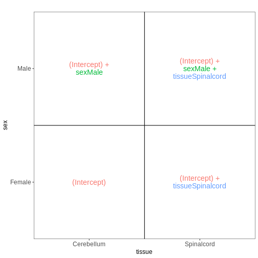
Factorial design with interactions
R
meta_noninf <- meta %>% filter(time == "Day0")
meta_noninf
OUTPUT
                     title geo_accession     organism     age    sex
GSM2545337 CNS_RNA-seq_11C    GSM2545337 Mus musculus 8 weeks Female
GSM2545338 CNS_RNA-seq_12C    GSM2545338 Mus musculus 8 weeks Female
GSM2545343 CNS_RNA-seq_20C    GSM2545343 Mus musculus 8 weeks   Male
GSM2545348 CNS_RNA-seq_27C    GSM2545348 Mus musculus 8 weeks Female
GSM2545349 CNS_RNA-seq_28C    GSM2545349 Mus musculus 8 weeks   Male
GSM2545353  CNS_RNA-seq_3C    GSM2545353 Mus musculus 8 weeks Female
GSM2545354  CNS_RNA-seq_4C    GSM2545354 Mus musculus 8 weeks   Male
GSM2545356 CNS_RNA-seq_574    GSM2545356 Mus musculus 8 weeks   Male
GSM2545357 CNS_RNA-seq_575    GSM2545357 Mus musculus 8 weeks   Male
GSM2545358 CNS_RNA-seq_583    GSM2545358 Mus musculus 8 weeks Female
GSM2545361 CNS_RNA-seq_590    GSM2545361 Mus musculus 8 weeks   Male
GSM2545364 CNS_RNA-seq_709    GSM2545364 Mus musculus 8 weeks Female
GSM2545365 CNS_RNA-seq_710    GSM2545365 Mus musculus 8 weeks Female
GSM2545366 CNS_RNA-seq_711    GSM2545366 Mus musculus 8 weeks Female
GSM2545367 CNS_RNA-seq_713    GSM2545367 Mus musculus 8 weeks   Male
             infection  strain time     tissue mouse
GSM2545337 NonInfected C57BL/6 Day0 Cerebellum     9
GSM2545338 NonInfected C57BL/6 Day0 Cerebellum    10
GSM2545343 NonInfected C57BL/6 Day0 Cerebellum    11
GSM2545348 NonInfected C57BL/6 Day0 Cerebellum     8
GSM2545349 NonInfected C57BL/6 Day0 Cerebellum     7
GSM2545353 NonInfected C57BL/6 Day0 Cerebellum     4
GSM2545354 NonInfected C57BL/6 Day0 Cerebellum     2
GSM2545356 NonInfected C57BL/6 Day0 Spinalcord     2
GSM2545357 NonInfected C57BL/6 Day0 Spinalcord     3
GSM2545358 NonInfected C57BL/6 Day0 Spinalcord     4
GSM2545361 NonInfected C57BL/6 Day0 Spinalcord     7
GSM2545364 NonInfected C57BL/6 Day0 Spinalcord     8
GSM2545365 NonInfected C57BL/6 Day0 Spinalcord     9
GSM2545366 NonInfected C57BL/6 Day0 Spinalcord    10
GSM2545367 NonInfected C57BL/6 Day0 Spinalcord    11
R
vd <- VisualizeDesign(sampleData = meta_noninf,
                      designFormula = ~ sex * tissue)
vd$designmatrix
OUTPUT
           (Intercept) sexMale tissueSpinalcord sexMale:tissueSpinalcord
GSM2545337           1       0                0                        0
GSM2545338           1       0                0                        0
GSM2545343           1       1                0                        0
GSM2545348           1       0                0                        0
GSM2545349           1       1                0                        0
GSM2545353           1       0                0                        0
GSM2545354           1       1                0                        0
GSM2545356           1       1                1                        1
GSM2545357           1       1                1                        1
GSM2545358           1       0                1                        0
GSM2545361           1       1                1                        1
GSM2545364           1       0                1                        0
GSM2545365           1       0                1                        0
GSM2545366           1       0                1                        0
GSM2545367           1       1                1                        1
R
vd$plotlist
OUTPUT
[[1]]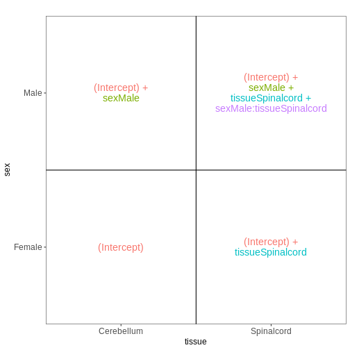
Paired design
R
meta_fem_day0 <- meta %>% filter(sex == "Female" &
                                     time == "Day0")
meta_fem_day0
OUTPUT
                     title geo_accession     organism     age    sex
GSM2545337 CNS_RNA-seq_11C    GSM2545337 Mus musculus 8 weeks Female
GSM2545338 CNS_RNA-seq_12C    GSM2545338 Mus musculus 8 weeks Female
GSM2545348 CNS_RNA-seq_27C    GSM2545348 Mus musculus 8 weeks Female
GSM2545353  CNS_RNA-seq_3C    GSM2545353 Mus musculus 8 weeks Female
GSM2545358 CNS_RNA-seq_583    GSM2545358 Mus musculus 8 weeks Female
GSM2545364 CNS_RNA-seq_709    GSM2545364 Mus musculus 8 weeks Female
GSM2545365 CNS_RNA-seq_710    GSM2545365 Mus musculus 8 weeks Female
GSM2545366 CNS_RNA-seq_711    GSM2545366 Mus musculus 8 weeks Female
             infection  strain time     tissue mouse
GSM2545337 NonInfected C57BL/6 Day0 Cerebellum     9
GSM2545338 NonInfected C57BL/6 Day0 Cerebellum    10
GSM2545348 NonInfected C57BL/6 Day0 Cerebellum     8
GSM2545353 NonInfected C57BL/6 Day0 Cerebellum     4
GSM2545358 NonInfected C57BL/6 Day0 Spinalcord     4
GSM2545364 NonInfected C57BL/6 Day0 Spinalcord     8
GSM2545365 NonInfected C57BL/6 Day0 Spinalcord     9
GSM2545366 NonInfected C57BL/6 Day0 Spinalcord    10
R
vd <- VisualizeDesign(sampleData = meta_fem_day0,
                      designFormula = ~ mouse + tissue)
vd$designmatrix
OUTPUT
           (Intercept) mouse tissueSpinalcord
GSM2545337           1     9                0
GSM2545338           1    10                0
GSM2545348           1     8                0
GSM2545353           1     4                0
GSM2545358           1     4                1
GSM2545364           1     8                1
GSM2545365           1     9                1
GSM2545366           1    10                1
R
vd$plotlist
OUTPUT
[[1]]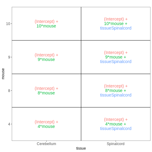
Within- and between-subject comparisons
R
meta_fem_day04 <- meta %>%
    filter(sex == "Female" &
               time %in% c("Day0", "Day4")) %>%
    droplevels()
meta_fem_day04
OUTPUT
                     title geo_accession     organism     age    sex
GSM2545337 CNS_RNA-seq_11C    GSM2545337 Mus musculus 8 weeks Female
GSM2545338 CNS_RNA-seq_12C    GSM2545338 Mus musculus 8 weeks Female
GSM2545339 CNS_RNA-seq_13C    GSM2545339 Mus musculus 8 weeks Female
GSM2545344 CNS_RNA-seq_21C    GSM2545344 Mus musculus 8 weeks Female
GSM2545348 CNS_RNA-seq_27C    GSM2545348 Mus musculus 8 weeks Female
GSM2545352 CNS_RNA-seq_30C    GSM2545352 Mus musculus 8 weeks Female
GSM2545353  CNS_RNA-seq_3C    GSM2545353 Mus musculus 8 weeks Female
GSM2545358 CNS_RNA-seq_583    GSM2545358 Mus musculus 8 weeks Female
GSM2545362  CNS_RNA-seq_5C    GSM2545362 Mus musculus 8 weeks Female
GSM2545364 CNS_RNA-seq_709    GSM2545364 Mus musculus 8 weeks Female
GSM2545365 CNS_RNA-seq_710    GSM2545365 Mus musculus 8 weeks Female
GSM2545366 CNS_RNA-seq_711    GSM2545366 Mus musculus 8 weeks Female
GSM2545371 CNS_RNA-seq_731    GSM2545371 Mus musculus 8 weeks Female
GSM2545375 CNS_RNA-seq_738    GSM2545375 Mus musculus 8 weeks Female
GSM2545376 CNS_RNA-seq_740    GSM2545376 Mus musculus 8 weeks Female
GSM2545377 CNS_RNA-seq_741    GSM2545377 Mus musculus 8 weeks Female
             infection  strain time     tissue mouse
GSM2545337 NonInfected C57BL/6 Day0 Cerebellum     9
GSM2545338 NonInfected C57BL/6 Day0 Cerebellum    10
GSM2545339  InfluenzaA C57BL/6 Day4 Cerebellum    15
GSM2545344  InfluenzaA C57BL/6 Day4 Cerebellum    22
GSM2545348 NonInfected C57BL/6 Day0 Cerebellum     8
GSM2545352  InfluenzaA C57BL/6 Day4 Cerebellum    21
GSM2545353 NonInfected C57BL/6 Day0 Cerebellum     4
GSM2545358 NonInfected C57BL/6 Day0 Spinalcord     4
GSM2545362  InfluenzaA C57BL/6 Day4 Cerebellum    20
GSM2545364 NonInfected C57BL/6 Day0 Spinalcord     8
GSM2545365 NonInfected C57BL/6 Day0 Spinalcord     9
GSM2545366 NonInfected C57BL/6 Day0 Spinalcord    10
GSM2545371  InfluenzaA C57BL/6 Day4 Spinalcord    15
GSM2545375  InfluenzaA C57BL/6 Day4 Spinalcord    20
GSM2545376  InfluenzaA C57BL/6 Day4 Spinalcord    21
GSM2545377  InfluenzaA C57BL/6 Day4 Spinalcord    22
R
design <- model.matrix(~ mouse, data = meta_fem_day04)
design <- cbind(design,
                Spc.Day0 = meta_fem_day04$tissue == "Spinalcord" &
                    meta_fem_day04$time == "Day0",
                Spc.Day4 = meta_fem_day04$tissue == "Spinalcord" &
                    meta_fem_day04$time == "Day4")
rownames(design) <- rownames(meta_fem_day04)
design
OUTPUT
           (Intercept) mouse Spc.Day0 Spc.Day4
GSM2545337           1     9        0        0
GSM2545338           1    10        0        0
GSM2545339           1    15        0        0
GSM2545344           1    22        0        0
GSM2545348           1     8        0        0
GSM2545352           1    21        0        0
GSM2545353           1     4        0        0
GSM2545358           1     4        1        0
GSM2545362           1    20        0        0
GSM2545364           1     8        1        0
GSM2545365           1     9        1        0
GSM2545366           1    10        1        0
GSM2545371           1    15        0        1
GSM2545375           1    20        0        1
GSM2545376           1    21        0        1
GSM2545377           1    22        0        1
R
vd <- VisualizeDesign(sampleData = meta_fem_day04 %>%
                          select(time, tissue, mouse),
                      designFormula = NULL,
                      designMatrix = design, flipCoordFitted = FALSE)
vd$designmatrix
OUTPUT
           (Intercept) mouse Spc.Day0 Spc.Day4
GSM2545337           1     9        0        0
GSM2545338           1    10        0        0
GSM2545339           1    15        0        0
GSM2545344           1    22        0        0
GSM2545348           1     8        0        0
GSM2545352           1    21        0        0
GSM2545353           1     4        0        0
GSM2545358           1     4        1        0
GSM2545362           1    20        0        0
GSM2545364           1     8        1        0
GSM2545365           1     9        1        0
GSM2545366           1    10        1        0
GSM2545371           1    15        0        1
GSM2545375           1    20        0        1
GSM2545376           1    21        0        1
GSM2545377           1    22        0        1
R
vd$plotlist
OUTPUT
$`time = Day0`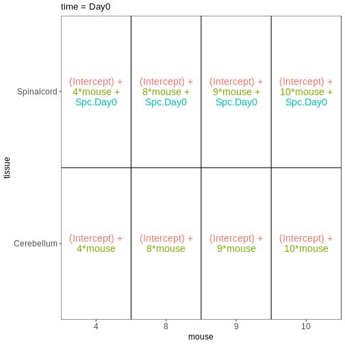
OUTPUT
$`time = Day4`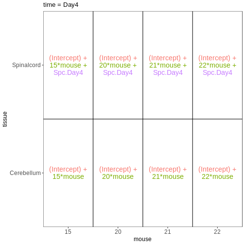
Content from Importing and annotating quantified data into R
Last updated on 2023-03-14 | Edit this page
Overview
Questions
- How do we get our data into R?
Objectives
- Learn how to import the quantifications into a SummarizedExperiment object.
- Learn how to add additional gene annotations to the object.
Contribute!
This episode is intended to show how we can assemble a SummarizedExperiment starting from individual count, rowdata and coldata files. Moreover, we will practice adding annotations for the genes, and discuss related concepts and things to keep in mind (annotation sources, versions, ‘helper’ packages like tximeta).
Read the data
Gene annotations
Need to be careful - the descriptions contain both commas and ’ (e.g., 5’)
R
rowranges <- read.delim("data/GSE96870_rowranges.tsv", sep = "\t",
                        colClasses = c(ENTREZID = "character"),
                        header = TRUE, quote = "", row.names = 5)
Mention other ways of getting annotations, and practice querying org package. Important to use the right annotation source/version.
R
suppressPackageStartupMessages({
    library(org.Mm.eg.db)
})
mapIds(org.Mm.eg.db, keys = "497097", column = "SYMBOL", keytype = "ENTREZID")
OUTPUT
'select()' returned 1:1 mapping between keys and columnsOUTPUT
497097
"Xkr4"
Check feature types
R
table(rowranges$gbkey)
OUTPUT
     C_region     D_segment          exon     J_segment      misc_RNA
           20            23          4008            94          1988
         mRNA         ncRNA precursor_RNA          rRNA          tRNA
        21198         12285          1187            35           413
    V_segment
          535
Assemble SummarizedExperiment
R
stopifnot(rownames(rowranges) == rownames(counts),
          rownames(coldata) == colnames(counts))

se <- SummarizedExperiment(
    assays = list(counts = as.matrix(counts)),
    rowRanges = as(rowranges, "GRanges"),
    colData = coldata
)
Save SummarizedExperiment
R
saveRDS(se, "data/GSE96870_se.rds")
Session info
R
sessionInfo()
OUTPUT
R version 4.2.2 Patched (2022-11-10 r83330)
Platform: x86_64-pc-linux-gnu (64-bit)
Running under: Ubuntu 22.04.2 LTS

Matrix products: default
BLAS:   /usr/lib/x86_64-linux-gnu/blas/libblas.so.3.10.0
LAPACK: /usr/lib/x86_64-linux-gnu/lapack/liblapack.so.3.10.0

locale:
 [1] LC_CTYPE=C.UTF-8       LC_NUMERIC=C           LC_TIME=C.UTF-8
 [4] LC_COLLATE=C.UTF-8     LC_MONETARY=C.UTF-8    LC_MESSAGES=C.UTF-8
 [7] LC_PAPER=C.UTF-8       LC_NAME=C              LC_ADDRESS=C
[10] LC_TELEPHONE=C         LC_MEASUREMENT=C.UTF-8 LC_IDENTIFICATION=C

attached base packages:
[1] stats4    stats     graphics  grDevices utils     datasets  methods
[8] base

other attached packages:
 [1] org.Mm.eg.db_3.16.0         AnnotationDbi_1.60.0
 [3] SummarizedExperiment_1.28.0 Biobase_2.58.0
 [5] MatrixGenerics_1.10.0       matrixStats_0.63.0
 [7] GenomicRanges_1.50.2        GenomeInfoDb_1.34.9
 [9] IRanges_2.32.0              S4Vectors_0.36.1
[11] BiocGenerics_0.44.0

loaded via a namespace (and not attached):
 [1] Rcpp_1.0.10            compiler_4.2.2         BiocManager_1.30.19
 [4] XVector_0.38.0         bitops_1.0-7           tools_4.2.2
 [7] zlibbioc_1.44.0        bit_4.0.5              RSQLite_2.2.20
[10] evaluate_0.20          memoise_2.0.1          lattice_0.20-45
[13] pkgconfig_2.0.3        png_0.1-8              rlang_1.0.6
[16] Matrix_1.5-3           DelayedArray_0.24.0    DBI_1.1.3
[19] cli_3.6.0              xfun_0.37              fastmap_1.1.0
[22] GenomeInfoDbData_1.2.9 httr_1.4.4             knitr_1.42
[25] Biostrings_2.66.0      vctrs_0.5.2            bit64_4.0.5
[28] grid_4.2.2             R6_2.5.1               blob_1.2.3
[31] KEGGREST_1.38.0        renv_0.17.0-38         RCurl_1.98-1.10
[34] cachem_1.0.6 crayon_1.5.2 Content from Exploratory analysis and quality control
Last updated on 2023-03-14 | Edit this page
Overview
Questions
Objectives
- Learn how to explore the gene expression matrix and perform common quality control steps.
- Learn how to set up an interactive application for exploratory analysis.
R
suppressPackageStartupMessages({
    library(SummarizedExperiment)
    library(DESeq2)
    library(vsn)
    library(ggplot2)
    library(ComplexHeatmap)
    library(RColorBrewer)
    library(hexbin)
})
R
se <- readRDS("data/GSE96870_se.rds")
Exploratory analysis is crucial for quality control and to get to know our data. It can help us detect quality problems, sample swaps and contamination, as well as give us a sense of the most salient patterns present in the data. In this episode, we will learn about two common ways of performing exploratory analysis for RNA-seq data; namely clustering and principal component analysis (PCA). These tools are in no way limited to (or developed for) analysis of RNA-seq data. However, there are certain characteristics of count assays that need to be taken into account when they are applied to this type of data.
R
se <- se[rowSums(assay(se, "counts")) > 5, ]
dds <- DESeq2::DESeqDataSet(se[, se$tissue == "Cerebellum"],
                            design = ~ sex + time)
WARNING
Warning in DESeq2::DESeqDataSet(se[, se$tissue == "Cerebellum"], design = ~sex
+ : some variables in design formula are characters, converting to factors
Library size differences
R
ggplot(data.frame(sample = colnames(dds),
                  libSize = colSums(assay(dds, "counts"))),
       aes(x = sample, y = libSize)) +
    geom_bar(stat = "identity") + theme_bw() +
    labs(x = "Sample", y = "Total count") +
    theme(axis.text.x = element_text(angle = 90, hjust = 1, vjust = 0.5))
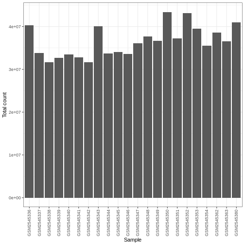
Differences in the total number of reads assigned to genes between samples typically occur for technical reasons. In practice, it means that we can not simply compare the raw read count directly between samples and conclude that a sample with a higher read count also expresses the gene more strongly - the higher count may be caused by an overall higher number of reads in that sample. In the rest of this section, we will use the term library size to refer to the total number of reads assigned to genes for a sample. We need to adjust for the differences in library size between samples, to avoid drawing incorrect conclusions. The way this is typically done for RNA-seq data can be described as a two-step procedure. First, we estimate size factors - sample-specific correction factors such that if the raw counts were to be divided by these factors, the resulting values would be more comparable across samples. Next, these size factors are incorporated into the statistical analysis of the data. It is important to pay close attention to how this is done in practice for a given analysis method. Sometimes the division of the counts by the size factors needs to be done explicitly by the analyst. Other times (as we will see for the differential expression analysis) it is important that they are provided separately to the analysis tool, which will then use them appropriately in the statistical model.
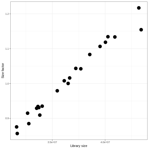
With DESeq2, size factors are calculated using the
estimateSizeFactors() function. The size factors estimated
by this function combines an adjustment for differences in library sizes
with an adjustment for differences in the RNA composition of the
samples. The latter is important due to the compositional nature of
RNA-seq data. There is a fixed number of reads to distribute between the
genes, and if a single (or a few) very highly expressed gene consume a
large part of the reads, all other genes will consequently receive very
low counts.
R
dds <- estimateSizeFactors(dds)
ggplot(data.frame(libSize = colSums(assay(dds, "counts")),
                  sizeFactor = sizeFactors(dds)),
       aes(x = libSize, y = sizeFactor)) +
    geom_point(size = 5) + theme_bw() +
    labs(x = "Library size", y = "Size factor")
Transform data
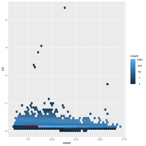
There is a rich literature on methods for exploratory analysis. Most of these work best in situations where the variance of the input data (here, each gene) is relatively independent of the average value. For read count data such as RNA-seq, this is not the case. In fact, the variance increases with the average read count.
R
meanSdPlot(assay(dds), ranks = FALSE)
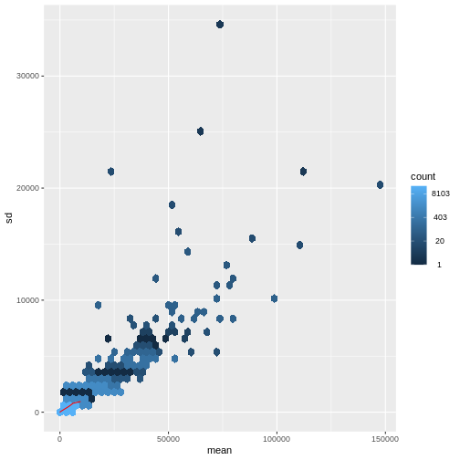
There are two ways around this: either we develop methods specifically adapted to count data, or we adapt (transform) the count data so that the existing methods are applicable. Both ways have been explored; however, at the moment the second approach is arguably more widely applied in practice.
R
vsd <- DESeq2::vst(dds, blind = TRUE)
meanSdPlot(assay(vsd), ranks = FALSE)
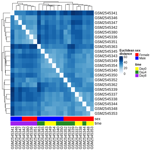
Heatmaps and clustering
R
dst <- dist(t(assay(vsd)))
colors <- colorRampPalette(brewer.pal(9, "Blues"))(255)
ComplexHeatmap::Heatmap(
    as.matrix(dst),
    col = colors,
    name = "Euclidean\ndistance",
    cluster_rows = hclust(dst),
    cluster_columns = hclust(dst),
    bottom_annotation = columnAnnotation(
        sex = vsd$sex,
        time = vsd$time,
        col = list(sex = c(Female = "red", Male = "blue"),
                   time = c(Day0 = "yellow", Day4 = "forestgreen", Day8 = "purple")))
)
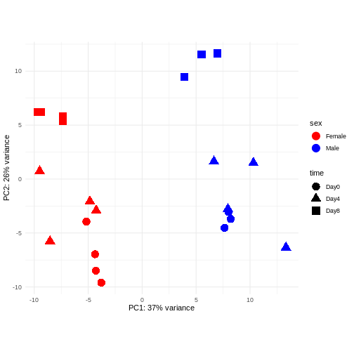
PCA
Principal component analysis is a dimensionality reduction method, which projects the samples into a lower-dimensional space. This lower-dimensional representation can be used for visualization, or as the input for other analysis methods. The principal components are defined in such a way that they are orthogonal, and that the projection of the samples into the space they span contains as much variance as possible. It is an unsupervised method in the sense that no external information about the samples (e.g., the treatment condition) is taken into account. In the plot below we represent the samples in a two-dimensional principal component space. For each of the two dimensions, we indicate the fraction of the total variance that is represented by that component. By definition, the first principal component will always represent more of the variance than the subsequent ones. The fraction of explained variance is a measure of how much of the ‘signal’ in the data that is retained when we project the samples from the original, high-dimensional space to the low-dimensional space for visualization.
R
pcaData <- DESeq2::plotPCA(vsd, intgroup = c("sex", "time"),
                           returnData = TRUE)
percentVar <- round(100 * attr(pcaData, "percentVar"))
ggplot(pcaData, aes(x = PC1, y = PC2)) +
    geom_point(aes(color = sex, shape = time), size = 5) +
    theme_minimal() +
    xlab(paste0("PC1: ", percentVar[1], "% variance")) +
    ylab(paste0("PC2: ", percentVar[2], "% variance")) +
    coord_fixed() +
    scale_color_manual(values = c(Male = "blue", Female = "red"))
Session info
R
sessionInfo()
OUTPUT
R version 4.2.2 Patched (2022-11-10 r83330)
Platform: x86_64-pc-linux-gnu (64-bit)
Running under: Ubuntu 22.04.2 LTS

Matrix products: default
BLAS:   /usr/lib/x86_64-linux-gnu/blas/libblas.so.3.10.0
LAPACK: /usr/lib/x86_64-linux-gnu/lapack/liblapack.so.3.10.0

locale:
 [1] LC_CTYPE=C.UTF-8       LC_NUMERIC=C           LC_TIME=C.UTF-8
 [4] LC_COLLATE=C.UTF-8     LC_MONETARY=C.UTF-8    LC_MESSAGES=C.UTF-8
 [7] LC_PAPER=C.UTF-8       LC_NAME=C              LC_ADDRESS=C
[10] LC_TELEPHONE=C         LC_MEASUREMENT=C.UTF-8 LC_IDENTIFICATION=C

attached base packages:
[1] grid      stats4    stats     graphics  grDevices utils     datasets
[8] methods   base

other attached packages:
 [1] hexbin_1.28.2               RColorBrewer_1.1-3
 [3] ComplexHeatmap_2.14.0       ggplot2_3.4.0
 [5] vsn_3.66.0                  DESeq2_1.38.3
 [7] SummarizedExperiment_1.28.0 Biobase_2.58.0
 [9] MatrixGenerics_1.10.0       matrixStats_0.63.0
[11] GenomicRanges_1.50.2        GenomeInfoDb_1.34.9
[13] IRanges_2.32.0              S4Vectors_0.36.1
[15] BiocGenerics_0.44.0

loaded via a namespace (and not attached):
 [1] httr_1.4.4             bit64_4.0.5            foreach_1.5.2
 [4] highr_0.10             BiocManager_1.30.19    affy_1.76.0
 [7] blob_1.2.3             renv_0.17.0-38         GenomeInfoDbData_1.2.9
[10] pillar_1.8.1           RSQLite_2.2.20         lattice_0.20-45
[13] glue_1.6.2             limma_3.54.1           digest_0.6.31
[16] XVector_0.38.0         colorspace_2.1-0       preprocessCore_1.60.2
[19] Matrix_1.5-3           XML_3.99-0.13          pkgconfig_2.0.3
[22] GetoptLong_1.0.5       zlibbioc_1.44.0        xtable_1.8-4
[25] scales_1.2.1           affyio_1.68.0          BiocParallel_1.32.5
[28] tibble_3.1.8           annotate_1.76.0        KEGGREST_1.38.0
[31] farver_2.1.1           generics_0.1.3         cachem_1.0.6
[34] withr_2.5.0            cli_3.6.0              magrittr_2.0.3
[37] crayon_1.5.2           memoise_2.0.1          evaluate_0.20
[40] fansi_1.0.4            doParallel_1.0.17      tools_4.2.2
[43] GlobalOptions_0.1.2    lifecycle_1.0.3        munsell_0.5.0
[46] locfit_1.5-9.7         cluster_2.1.4          DelayedArray_0.24.0
[49] AnnotationDbi_1.60.0   Biostrings_2.66.0      compiler_4.2.2
[52] rlang_1.0.6            RCurl_1.98-1.10        iterators_1.0.14
[55] circlize_0.4.15        rjson_0.2.21           labeling_0.4.2
[58] bitops_1.0-7           gtable_0.3.1           codetools_0.2-19
[61] DBI_1.1.3              R6_2.5.1               knitr_1.42
[64] dplyr_1.1.0            fastmap_1.1.0          bit_4.0.5
[67] utf8_1.2.3             clue_0.3-64            shape_1.4.6
[70] parallel_4.2.2         Rcpp_1.0.10            vctrs_0.5.2
[73] geneplotter_1.76.0     png_0.1-8              tidyselect_1.2.0
[76] xfun_0.37 Content from Differential expression analysis
Last updated on 2023-03-14 | Edit this page
Overview
Questions
- How do we find differentially expressed genes?
Objectives
- Explain the steps involved in a differential expression analysis.
- Explain how to perform these steps in R, using DESeq2.
R
suppressPackageStartupMessages({
    library(SummarizedExperiment)
    library(DESeq2)
    library(ggplot2)
    library(ExploreModelMatrix)
    library(cowplot)
    library(ComplexHeatmap)
})
Load data
R
se <- readRDS("data/GSE96870_se.rds")
Create DESeqDataSet
R
dds <- DESeq2::DESeqDataSet(se[, se$tissue == "Cerebellum"],
                            design = ~ sex + time)
WARNING
Warning in DESeq2::DESeqDataSet(se[, se$tissue == "Cerebellum"], design = ~sex
+ : some variables in design formula are characters, converting to factors
Run DESeq()
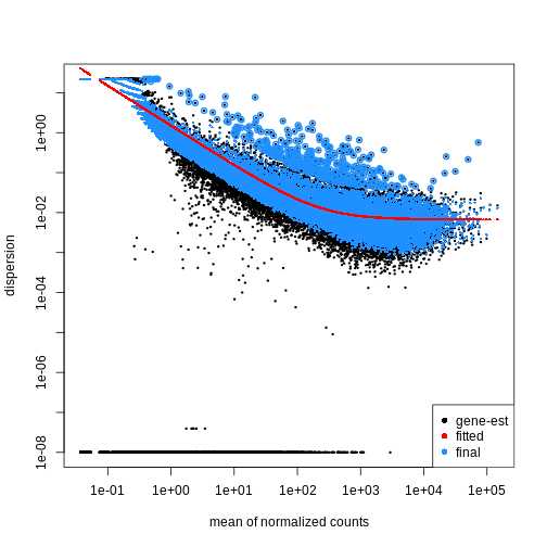
R
dds <- DESeq2::DESeq(dds)
OUTPUT
estimating size factorsOUTPUT
estimating dispersionsOUTPUT
gene-wise dispersion estimatesOUTPUT
mean-dispersion relationshipOUTPUT
final dispersion estimatesOUTPUT
fitting model and testingR
plotDispEsts(dds)
Extract results for specific contrasts
R
## Day 8 vs Day 0
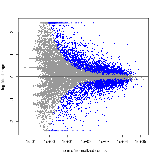
resTime <- DESeq2::results(dds, contrast = c("time", "Day8", "Day0"))
summary(resTime)
OUTPUT
out of 32652 with nonzero total read count
adjusted p-value < 0.1
LFC > 0 (up)       : 4472, 14%
LFC < 0 (down)     : 4276, 13%
outliers [1]       : 10, 0.031%
low counts [2]     : 8732, 27%
(mean count < 1)
[1] see 'cooksCutoff' argument of ?results
[2] see 'independentFiltering' argument of ?results
R
head(resTime[order(resTime$pvalue), ])
OUTPUT
log2 fold change (MLE): time Day8 vs Day0
Wald test p-value: time Day8 vs Day0
DataFrame with 6 rows and 6 columns
               baseMean log2FoldChange     lfcSE      stat      pvalue
              <numeric>      <numeric> <numeric> <numeric>   <numeric>
Asl             701.343        1.11733 0.0592541   18.8565 2.59885e-79
Apod          18765.146        1.44698 0.0805186   17.9708 3.30147e-72
Cyp2d22        2550.480        0.91020 0.0554756   16.4072 1.69794e-60
Klk6            546.503       -1.67190 0.1058989  -15.7877 3.78228e-56
Fcrls           184.235       -1.94701 0.1279847  -15.2128 2.90708e-52
A330076C08Rik   107.250       -1.74995 0.1154279  -15.1606 6.45112e-52
                     padj
                <numeric>
Asl           6.21386e-75
Apod          3.94690e-68
Cyp2d22       1.35326e-56
Klk6          2.26086e-52
Fcrls         1.39017e-48
A330076C08Rik 2.57077e-48
R
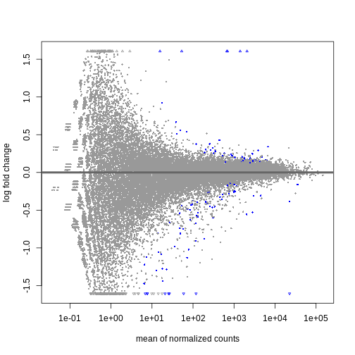
DESeq2::plotMA(resTime)
R
## Male vs Female
resSex <- DESeq2::results(dds, contrast = c("sex", "Male", "Female"))
summary(resSex)
OUTPUT
out of 32652 with nonzero total read count
adjusted p-value < 0.1
LFC > 0 (up)       : 53, 0.16%
LFC < 0 (down)     : 71, 0.22%
outliers [1]       : 10, 0.031%
low counts [2]     : 13717, 42%
(mean count < 6)
[1] see 'cooksCutoff' argument of ?results
[2] see 'independentFiltering' argument of ?results
R
head(resSex[order(resSex$pvalue), ])
OUTPUT
log2 fold change (MLE): sex Male vs Female
Wald test p-value: sex Male vs Female
DataFrame with 6 rows and 6 columns
               baseMean log2FoldChange     lfcSE      stat       pvalue
              <numeric>      <numeric> <numeric> <numeric>    <numeric>
Xist         22603.0359      -11.60429  0.336282  -34.5076 6.16852e-261
Ddx3y         2072.9436       11.87241  0.397493   29.8683 5.08722e-196
Eif2s3y       1410.8750       12.62514  0.565216   22.3369 1.62066e-110
Kdm5d          692.1672       12.55386  0.593627   21.1477  2.89566e-99
Uty            667.4375       12.01728  0.593591   20.2451  3.92780e-91
LOC105243748    52.9669        9.08325  0.597624   15.1989  3.59432e-52
                     padj
                <numeric>
Xist         1.16739e-256
Ddx3y        4.81378e-192
Eif2s3y      1.02237e-106
Kdm5d         1.37001e-95
Uty           1.48667e-87
LOC105243748  1.13371e-48
R
DESeq2::plotMA(resSex)
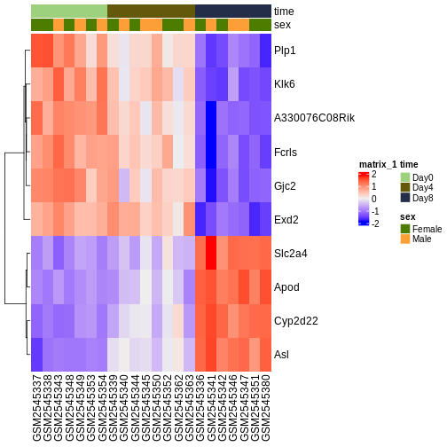
Visualize selected set of genes
R
vsd <- DESeq2::vst(dds, blind = TRUE)

genes <- rownames(head(resTime[order(resTime$pvalue), ], 10))
heatmapData <- assay(vsd)[genes, ]
heatmapData <- t(scale(t(heatmapData)))
heatmapColAnnot <- data.frame(colData(vsd)[, c("time", "sex")])
idx <- order(vsd$time)
heatmapData <- heatmapData[, idx]
heatmapColAnnot <- HeatmapAnnotation(df = heatmapColAnnot[idx, ])
ComplexHeatmap::Heatmap(heatmapData,
                        top_annotation = heatmapColAnnot,
                        cluster_rows = TRUE, cluster_columns = FALSE)
Content from Gene set analysis
Last updated on 2023-03-14 | Edit this page
Overview
Questions
- How do we find differentially expressed pathways?
Objectives
- Explain how to find differentially expressed pathways with gene set analysis in R.
- Understand how differentially expressed genes can enrich a gene set.
- Explain how to perform a gene set analysis in R, using clusterProfiler.
First, we are going to explore the basic concept of enriching a gene set with differentially expressed (DE) genes. Recall the differential expression analysis.
R
library(SummarizedExperiment)
library(DESeq2)
R
se <- readRDS("data/GSE96870_se.rds")
R
dds <- DESeq2::DESeqDataSet(se[, se$tissue == "Cerebellum"],
                            design = ~ sex + time)
WARNING
Warning in DESeq2::DESeqDataSet(se[, se$tissue == "Cerebellum"], design = ~sex
+ : some variables in design formula are characters, converting to factors
R
dds <- DESeq2::DESeq(dds)
Fetch results for the contrast between male and female mice.
R
resSex <- DESeq2::results(dds, contrast = c("sex", "Male", "Female"))
summary(resSex)
OUTPUT
out of 32652 with nonzero total read count
adjusted p-value < 0.1
LFC > 0 (up)       : 53, 0.16%
LFC < 0 (down)     : 71, 0.22%
outliers [1]       : 10, 0.031%
low counts [2]     : 13717, 42%
(mean count < 6)
[1] see 'cooksCutoff' argument of ?results
[2] see 'independentFiltering' argument of ?results
Select DE genes between males and females with FDR < 5%.
R
sexDE <- as.data.frame(subset(resSex, padj < 0.05))
dim(sexDE)
OUTPUT
[1] 54 6R
sexDE <- sexDE[order(abs(sexDE$log2FoldChange), decreasing=TRUE), ]
head(sexDE)
OUTPUT
               baseMean log2FoldChange     lfcSE      stat        pvalue
Eif2s3y       1410.8750       12.62514 0.5652155  22.33685 1.620659e-110
Kdm5d          692.1672       12.55386 0.5936267  21.14773  2.895664e-99
Uty            667.4375       12.01728 0.5935911  20.24505  3.927797e-91
Ddx3y         2072.9436       11.87241 0.3974927  29.86825 5.087220e-196
Xist         22603.0359      -11.60429 0.3362822 -34.50761 6.168523e-261
LOC105243748    52.9669        9.08325 0.5976242  15.19893  3.594320e-52
                      padj
Eif2s3y      1.022366e-106
Kdm5d         1.370011e-95
Uty           1.486671e-87
Ddx3y        4.813782e-192
Xist         1.167393e-256
LOC105243748  1.133708e-48
R
sexDEgenes <- rownames(sexDE)
head(sexDEgenes)
OUTPUT
[1] "Eif2s3y"      "Kdm5d"        "Uty"          "Ddx3y"        "Xist"
[6] "LOC105243748"
R
length(sexDEgenes)
OUTPUT
[1] 54Enrichment of a curated gene set
Contribute!
Here we illustrate how to assess the enrichment of one gene set we curate ourselves with our subset of DE genes with sex-specific expression. Here we form such a gene set with genes from sex chromosomes. Could you think of another more accurate gene set formed by genes with sex-specific expression?
Build a gene set formed by genes located in the sex chromosomes X and Y.
R
xygenes <- rownames(se)[decode(seqnames(rowRanges(se)) %in% c("X", "Y"))]
length(xygenes)
OUTPUT
[1] 2123Build a contingency table and conduct a one-tailed Fisher’s exact test that verifies the association between genes being DE between male and female mice and being located in a sex chromosome.
R
N <- nrow(se)
n <- length(sexDEgenes)
m <- length(xygenes)
k <- length(intersect(xygenes, sexDEgenes))
dnames <- list(GS=c("inside", "outside"), DE=c("yes", "no"))
t <- matrix(c(k, n-k, m-k, N+k-n-m),
                        nrow=2, ncol=2, dimnames=dnames)
t
OUTPUT
         DE
GS        yes    no
  inside   18  2105
  outside  36 39627
R
fisher.test(t, alternative="greater")
OUTPUT
	Fisher's Exact Test for Count Data

data:  t
p-value = 7.944e-11
alternative hypothesis: true odds ratio is greater than 1
95 percent confidence interval:
 5.541517      Inf
sample estimates:
odds ratio
  9.411737
Gene ontology analysis with clusterProfiler
Contribute!
Here we illustrate how to assess the enrichment on the entire collection of Gene Ontology (GO) gene sets using the package clusterProfiler. Could we illustrate any missing important feature of this package for this analysis objective? Could we briefly mention other packages that may be useful for this task?
Second, let’s perform a gene set analysis for an entire collection of gene sets using the Bioconductor package clusterProfiler. For this purpose, we will fetch the results for the contrast between two time points.
R
resTime <- DESeq2::results(dds, contrast = c("time", "Day8", "Day0"))
summary(resTime)
OUTPUT
out of 32652 with nonzero total read count
adjusted p-value < 0.1
LFC > 0 (up)       : 4472, 14%
LFC < 0 (down)     : 4276, 13%
outliers [1]       : 10, 0.031%
low counts [2]     : 8732, 27%
(mean count < 1)
[1] see 'cooksCutoff' argument of ?results
[2] see 'independentFiltering' argument of ?results
Select DE genes between Day0 and Day8 with
FDR < 5% and minimum 1.5-fold change.
R
timeDE <- as.data.frame(subset(resTime, padj < 0.05 & abs(log2FoldChange) > log2(1.5)))
dim(timeDE)
OUTPUT
[1] 2110 6R
timeDE <- timeDE[order(abs(timeDE$log2FoldChange), decreasing=TRUE), ]
head(timeDE)
OUTPUT
              baseMean log2FoldChange     lfcSE      stat       pvalue
LOC105245444  2.441873       4.768938 0.9013067  5.291138 1.215573e-07
LOC105246405  9.728219       4.601505 0.6101832  7.541186 4.657174e-14
4933427D06Rik 1.480365       4.556126 1.0318402  4.415535 1.007607e-05
A930006I01Rik 2.312732      -4.353155 0.9176026 -4.744053 2.094837e-06
LOC105245223  3.272536       4.337202 0.8611255  5.036666 4.737099e-07
A530053G22Rik 1.554735       4.243903 1.0248977  4.140806 3.460875e-05
                      padj
LOC105245444  1.800765e-06
LOC105246405  2.507951e-12
4933427D06Rik 9.169093e-05
A930006I01Rik 2.252139e-05
LOC105245223  6.047199e-06
A530053G22Rik 2.720142e-04
R
timeDEgenes <- rownames(timeDE)
head(timeDEgenes)
OUTPUT
[1] "LOC105245444"  "LOC105246405"  "4933427D06Rik" "A930006I01Rik"
[5] "LOC105245223"  "A530053G22Rik"
R
length(timeDEgenes)
OUTPUT
[1] 2110Call the enrichGO() function from clusterProfiler
as follows.
R
library(clusterProfiler)
library(org.Mm.eg.db)
library(enrichplot)

resTimeGO <- enrichGO(gene = timeDEgenes,
                      keyType = "SYMBOL",
                      universe = rownames(se),
                      OrgDb = org.Mm.eg.db,
                      ont = "BP",
                      pvalueCutoff = 0.01,
                      qvalueCutoff = 0.01)
dim(resTimeGO)
OUTPUT
[1] 17 9R
head(resTimeGO)
OUTPUT
                   ID                                           Description
GO:0035456 GO:0035456                           response to interferon-beta
GO:0071674 GO:0071674                            mononuclear cell migration
GO:0035458 GO:0035458                  cellular response to interferon-beta
GO:0050900 GO:0050900                                   leukocyte migration
GO:0030595 GO:0030595                                  leukocyte chemotaxis
GO:0002523 GO:0002523 leukocyte migration involved in inflammatory response
           GeneRatio   BgRatio       pvalue     p.adjust       qvalue
GO:0035456   17/1260  54/21417 6.434058e-09 3.254347e-05 3.082930e-05
GO:0071674   32/1260 179/21417 1.596474e-08 4.037482e-05 3.824814e-05
GO:0035458   15/1260  47/21417 4.064983e-08 6.749342e-05 6.393832e-05
GO:0050900   50/1260 375/21417 5.337558e-08 6.749342e-05 6.393832e-05
GO:0030595   34/1260 222/21417 2.880367e-07 2.913780e-04 2.760302e-04
GO:0002523   10/1260  25/21417 6.944905e-07 5.854555e-04 5.546176e-04
                                                                                                                                                                                                                                                                                             geneID
GO:0035456                                                                                                                                                                            Tgtp1/Tgtp2/F830016B08Rik/Iigp1/Ifitm6/Igtp/Gm4951/Bst2/Oas1c/Irgm1/Gbp6/Ifi47/Aim2/Ifitm7/Irgm2/Ifit1/Ifi204
GO:0071674                                                                                                    Tnfsf18/Aire/Ccl17/Ccr7/Nlrp12/Ccl2/Retnlg/Apod/Il12a/Ccl5/Fut7/Ccl7/Spn/Itgb3/Grem1/Ptk2b/Lgals3/Adam8/Dusp1/Ch25h/Nbl1/Alox5/Padi2/Plg/Calr/Ager/Slamf9/Ccl6/Mdk/Itga4/Hsd3b7/Trpm4
GO:0035458                                                                                                                                                                                        Tgtp1/Tgtp2/F830016B08Rik/Iigp1/Igtp/Gm4951/Oas1c/Irgm1/Gbp6/Ifi47/Aim2/Ifitm7/Irgm2/Ifit1/Ifi204
GO:0050900 Tnfsf18/Aire/Ccl17/Ccr7/Nlrp12/Bst1/Ccl2/Retnlg/Ppbp/Cxcl5/Apod/Il12a/Ccl5/Umodl1/Fut7/Ccl7/Ccl28/Spn/Sell/Itgb3/Grem1/Cxcl1/Ptk2b/Lgals3/Adam8/Pf4/Dusp1/Ch25h/S100a8/Nbl1/Alox5/Padi2/Plg/Edn3/Il33/Ptn/Ada/Enpp1/Calr/Ager/Slamf9/Ccl6/Prex1/Aoc3/Itgam/Mdk/Itga4/Hsd3b7/P2ry12/Trpm4
GO:0030595                                                                                        Tnfsf18/Ccl17/Ccr7/Bst1/Ccl2/Retnlg/Ppbp/Cxcl5/Il12a/Ccl5/Ccl7/Sell/Grem1/Cxcl1/Ptk2b/Lgals3/Adam8/Pf4/Dusp1/Ch25h/S100a8/Nbl1/Alox5/Padi2/Edn3/Ptn/Calr/Slamf9/Ccl6/Prex1/Itgam/Mdk/Hsd3b7/Trpm4
GO:0002523                                                                                                                                                                                                                                     Ccl2/Ppbp/Fut7/Adam8/S100a8/Alox5/Ptn/Aoc3/Itgam/Mdk
           Count
GO:0035456    17
GO:0071674    32
GO:0035458    15
GO:0050900    50
GO:0030595    34
GO:0002523    10
Let’s build a more readable table of results.
R
library(kableExtra)

resTimeGOtab <- as.data.frame(resTimeGO)
resTimeGOtab$ID <- NULL
resTimeGOtab$geneID <- sapply(strsplit(resTimeGO$geneID, "/"), paste, collapse=", ")
ktab <- kable(resTimeGOtab, row.names=TRUE, caption="GO results for DE genes between time points.")
kable_styling(ktab, bootstrap_options=c("stripped", "hover", "responsive"), fixed_thead=TRUE)
| Description | GeneRatio | BgRatio | pvalue | p.adjust | qvalue | geneID | Count | |
|---|---|---|---|---|---|---|---|---|
| GO:0035456 | response to interferon-beta | 17/1260 | 54/21417 | 0.00e+00 | 0.0000325 | 0.0000308 | Tgtp1, Tgtp2, F830016B08Rik, Iigp1, Ifitm6, Igtp, Gm4951, Bst2, Oas1c, Irgm1, Gbp6, Ifi47, Aim2, Ifitm7, Irgm2, Ifit1, Ifi204 | 17 |
| GO:0071674 | mononuclear cell migration | 32/1260 | 179/21417 | 0.00e+00 | 0.0000404 | 0.0000382 | Tnfsf18, Aire, Ccl17, Ccr7, Nlrp12, Ccl2, Retnlg, Apod, Il12a, Ccl5, Fut7, Ccl7, Spn, Itgb3, Grem1, Ptk2b, Lgals3, Adam8, Dusp1, Ch25h, Nbl1, Alox5, Padi2, Plg, Calr, Ager, Slamf9, Ccl6, Mdk, Itga4, Hsd3b7, Trpm4 | 32 |
| GO:0035458 | cellular response to interferon-beta | 15/1260 | 47/21417 | 0.00e+00 | 0.0000675 | 0.0000639 | Tgtp1, Tgtp2, F830016B08Rik, Iigp1, Igtp, Gm4951, Oas1c, Irgm1, Gbp6, Ifi47, Aim2, Ifitm7, Irgm2, Ifit1, Ifi204 | 15 |
| GO:0050900 | leukocyte migration | 50/1260 | 375/21417 | 1.00e-07 | 0.0000675 | 0.0000639 | Tnfsf18, Aire, Ccl17, Ccr7, Nlrp12, Bst1, Ccl2, Retnlg, Ppbp, Cxcl5, Apod, Il12a, Ccl5, Umodl1, Fut7, Ccl7, Ccl28, Spn, Sell, Itgb3, Grem1, Cxcl1, Ptk2b, Lgals3, Adam8, Pf4, Dusp1, Ch25h, S100a8, Nbl1, Alox5, Padi2, Plg, Edn3, Il33, Ptn, Ada, Enpp1, Calr, Ager, Slamf9, Ccl6, Prex1, Aoc3, Itgam, Mdk, Itga4, Hsd3b7, P2ry12, Trpm4 | 50 |
| GO:0030595 | leukocyte chemotaxis | 34/1260 | 222/21417 | 3.00e-07 | 0.0002914 | 0.0002760 | Tnfsf18, Ccl17, Ccr7, Bst1, Ccl2, Retnlg, Ppbp, Cxcl5, Il12a, Ccl5, Ccl7, Sell, Grem1, Cxcl1, Ptk2b, Lgals3, Adam8, Pf4, Dusp1, Ch25h, S100a8, Nbl1, Alox5, Padi2, Edn3, Ptn, Calr, Slamf9, Ccl6, Prex1, Itgam, Mdk, Hsd3b7, Trpm4 | 34 |
| GO:0002523 | leukocyte migration involved in inflammatory response | 10/1260 | 25/21417 | 7.00e-07 | 0.0005855 | 0.0005546 | Ccl2, Ppbp, Fut7, Adam8, S100a8, Alox5, Ptn, Aoc3, Itgam, Mdk | 10 |
| GO:0050953 | sensory perception of light stimulus | 26/1260 | 162/21417 | 2.90e-06 | 0.0020909 | 0.0019808 | Aipl1, Vsx2, Nxnl2, Lrit3, Cryba2, Bfsp2, Lrat, Gabrr2, Lum, Rlbp1, Pde6g, Gpr179, Col1a1, Cplx3, Best1, Ush1g, Rs1, Rdh5, Guca1b, Th, Ppef2, Rbp4, Olfm2, Rom1, Vsx1, Rpe65 | 26 |
| GO:0071675 | regulation of mononuclear cell migration | 21/1260 | 117/21417 | 4.20e-06 | 0.0026851 | 0.0025436 | Tnfsf18, Aire, Ccr7, Ccl2, Apod, Il12a, Ccl5, Ccl7, Spn, Itgb3, Grem1, Ptk2b, Lgals3, Adam8, Dusp1, Nbl1, Padi2, Calr, Ager, Mdk, Itga4 | 21 |
| GO:0007601 | visual perception | 25/1260 | 158/21417 | 5.80e-06 | 0.0032508 | 0.0030795 | Aipl1, Vsx2, Nxnl2, Lrit3, Cryba2, Bfsp2, Lrat, Gabrr2, Lum, Rlbp1, Pde6g, Gpr179, Col1a1, Cplx3, Best1, Rs1, Rdh5, Guca1b, Th, Ppef2, Rbp4, Olfm2, Rom1, Vsx1, Rpe65 | 25 |
| GO:0034341 | response to interferon-gamma | 22/1260 | 135/21417 | 1.28e-05 | 0.0056936 | 0.0053937 | Ccl17, Gbp4, Ccl2, Tgtp1, H2-Q7, Il12rb1, Ifitm6, Ccl5, Ccl7, Igtp, Nos2, Nlrc5, Bst2, Irgm1, Gbp6, Capg, Ifitm7, Gbp9, Gbp5, Irgm2, Ccl6, Aqp4 | 22 |
| GO:0060326 | cell chemotaxis | 38/1260 | 308/21417 | 1.30e-05 | 0.0056936 | 0.0053937 | Tnfsf18, Ccl17, Ccr7, Bst1, Ccl2, Retnlg, Ppbp, Cxcl5, Nr4a1, Il12a, Ccl5, Ccl7, Ccl28, Sell, Grem1, Cxcl1, Ptk2b, Lgals3, Adam8, Pf4, Dusp1, Ch25h, S100a8, Nbl1, Alox5, Padi2, Edn3, Ptn, Plxnb3, Calr, Lpar1, Slamf9, Ccl6, Prex1, Itgam, Mdk, Hsd3b7, Trpm4 | 38 |
| GO:0002685 | regulation of leukocyte migration | 31/1260 | 230/21417 | 1.41e-05 | 0.0056936 | 0.0053937 | Tnfsf18, Aire, Ccr7, Bst1, Ccl2, Apod, Il12a, Ccl5, Fut7, Ccl7, Ccl28, Spn, Sell, Itgb3, Grem1, Ptk2b, Lgals3, Adam8, Dusp1, Nbl1, Padi2, Edn3, Il33, Ptn, Ada, Calr, Ager, Aoc3, Mdk, Itga4, P2ry12 | 31 |
| GO:0036336 | dendritic cell migration | 9/1260 | 27/21417 | 1.46e-05 | 0.0056936 | 0.0053937 | Tnfsf18, Ccr7, Nlrp12, Retnlg, Il12a, Alox5, Calr, Slamf9, Trpm4 | 9 |
| GO:1990266 | neutrophil migration | 21/1260 | 127/21417 | 1.59e-05 | 0.0057426 | 0.0054401 | Ccl17, Ccr7, Bst1, Ccl2, Ppbp, Cxcl5, Ccl5, Umodl1, Fut7, Ccl7, Sell, Cxcl1, Lgals3, Adam8, Pf4, S100a8, Edn3, Ccl6, Prex1, Itgam, Mdk | 21 |
| GO:0016264 | gap junction assembly | 7/1260 | 16/21417 | 1.71e-05 | 0.0057811 | 0.0054766 | Gjd3, Aplnr, Gja5, Agt, Hopx, Cav1, Ace | 7 |
| GO:0030593 | neutrophil chemotaxis | 18/1260 | 100/21417 | 1.94e-05 | 0.0061338 | 0.0058107 | Ccl17, Ccr7, Bst1, Ccl2, Ppbp, Cxcl5, Ccl5, Ccl7, Sell, Cxcl1, Lgals3, Pf4, S100a8, Edn3, Ccl6, Prex1, Itgam, Mdk | 18 |
| GO:1903028 | positive regulation of opsonization | 6/1260 | 12/21417 | 2.78e-05 | 0.0082825 | 0.0078462 | Pla2g5, Masp2, C4b, Colec11, C3, Cfp | 6 |