Getting started with R Markdown (Optional)
Last updated on 2023-01-05 | Edit this page
Estimated time 45 minutes
Overview
Questions
- What is R Markdown?
- How can I integrate my R code with text and plots?
- How can I convert .Rmd files to .html?
Objectives
- Create a .Rmd document containing R code, text, and plots
- Create a YAML header to control output
- Understand basic syntax of (R)Markdown
- Customise code chunks to control formatting
- Use code chunks and in-line code to create dynamic, reproducible documents
R Markdown
R Markdown is a flexible type of document that allows you to seamlessly combine executable R code, and its output, with text in a single document. These documents can be readily converted to multiple static and dynamic output formats, including PDF (.pdf), Word (.docx), and HTML (.html).
The benefit of a well-prepared R Markdown document is full reproducibility. This also means that, if you notice a data transcription error, or you are able to add more data to your analysis, you will be able to recompile the report without making any changes in the actual document.
The rmarkdown package comes pre-installed with RStudio, so no action is necessary.
Creating an R Markdown file
To create a new R Markdown document in RStudio, click File -> New File -> R Markdown:
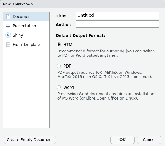
Then click on ‘Create Empty Document’. Normally you could enter the title of your document, your name (Author), and select the type of output, but we will be learning how to start from a blank document.
Basic components of R Markdown
To control the output, a YAML (YAML Ain’t Markup Language) header is needed:
---
title: "My Awesome Report"
author: "Emmet Brickowski"
date: ""
output: html_document
---
The header is defined by the three hyphens at the beginning
(---) and the three hyphens at the end
(---).
In the YAML, the only required field is the output:,
which specifies the type of output you want. This can be an
html_document, a pdf_document, or a
word_document. We will start with an HTML doument and
discuss the other options later.
The rest of the fields can be deleted, if you don’t need them. After
the header, to begin the body of the document, you start typing after
the end of the YAML header (i.e. after the second ---).
Markdown syntax
Markdown is a popular markup language that allows you to add
formatting elements to text, such as bold,
italics, and code. The formatting will not be
immediately visible in a markdown (.md) document, like you would see in
a Word document. Rather, you add Markdown syntax to the text, which can
then be converted to various other files that can translate the Markdown
syntax. Markdown is useful because it is lightweight, flexible, and
platform independent.
Some platforms provide a real time preview of the formatting, like RStudio’s visual markdown editor (available from version 1.4).
First, let’s create a heading! A # in front of text
indicates to Markdown that this text is a heading. Adding more
#s make the heading smaller, i.e. one # is a
first level heading, two ##s is a second level heading,
etc. upto the 6th level heading.
# Title
## Section
### Sub-section
#### Sub-sub section
##### Sub-sub-sub section
###### Sub-sub-sub-sub section
(only use a level if the one above is also in use)
Since we have already defined our title in the YAML header, we will use a section heading to create an Introduction section.
## IntroductionYou can make things bold by surrounding the word
with double asterisks, **bold**, or double underscores,
__bold__; and italicize using single asterisks,
*italics*, or single underscores,
_italics_.
You can also combine bold and italics to
write something really important with
triple-asterisks, ***really***, or underscores,
___really___; and, if you’re feeling bold (pun intended),
you can also use a combination of asterisks and underscores,
**_really_**, **_really_**.
To create code-type font, surround the word with
backticks, code-type.
Now that we’ve learned a couple of things, it might be useful to implement them:
## Introduction

This report uses the **tidyverse** package along with the *SAFI* dataset,
which has columns that include:
Then we can create a list for the variables using -,
+, or * keys.
## Introduction

This report uses the **tidyverse** package along with the *SAFI* dataset,
which has columns that include:

- village
- interview_date
- no_members
- years_liv
- respondent_wall_type
- rooms
You can also create an ordered list using numbers:
1. village
2. interview_date
3. no_members
4. years_liv
5. respondent_wall_type
6. rooms
And nested items by tab-indenting:
- village
  + Name of village
- interview_date
  + Date of interview
- no_members
  + How many family members lived in a house
- years_liv
  + How many years respondent has lived in village or neighbouring village
- respondent_wall_type
  + Type of wall of house
- rooms
  + Number of rooms in house
For more Markdown syntax see the following reference guide.
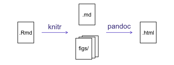
Now we can render the document into HTML by clicking the Knit button in the top of the Source pane (top left), or use the keyboard shortcut Ctrl+Shift+K on Windows and Linux, and Cmd+Shift+K on Mac. If you haven’t saved the document yet, you will be prompted to do so when you Knit for the first time.
Writing an R Markdown report
Now we will add some R code from our previous data wrangling and visualisation, which means we need to make sure tidyverse is loaded. It is not enough to load tidyverse from the console, we will need to load it within our R Markdown document. The same applies to our data. To load these, we will need to create a ‘code chunk’ at the top of our document (below the YAML header).
A code chunk can be inserted by clicking Code > Insert Chunk, or by using the keyboard shortcuts Ctrl+Alt+I on Windows and Linux, and Cmd+Option+I on Mac.
The syntax of a code chunk is:
```{r chunk-name}
Here is where you place the R code that you want to run.
```
An R Markdown document knows that this text is not part of the report
from the ``` that begins and ends
the chunk. It also knows that the code inside of the chunk is R code
from the r inside of the curly braces ({}).
After the r you can add a name for the code chunk . Naming
a chunk is optional, but recommended. Each chunk name must be unique,
and only contain alphanumeric characters and -.
To load tidyverse and our
SAFI_clean.csv file, we will insert a chunk and call it
‘setup’. Since we don’t want this code or the output to show in our
knitted HTML document, we add an include = FALSE option
after the code chunk name ({r setup, include = FALSE}).
```{r setup, include = FALSE}
library(tidyverse)
library(here)
interviews
Insert table
Next, we will re-create a table from the Data Wrangling episode which
shows the average household size grouped by village and
memb_assoc. We can do this by creating a new code chunk and
calling it ‘interview-tbl’. Or, you can come up with something more
creative (just remember to stick to the naming rules).
It isn’t necessary to Knit your document every time you want to see the output. Instead you can run the code chunk with the green triangle in the top right corner of the the chunk, or with the keyboard shortcuts: Ctrl+Alt+C on Windows and Linux, or Cmd+Option+C on Mac.
To make sure the table is formatted nicely in our output document, we
will need to use the kable() function from the
knitr package. The kable() function takes
the output of your R code and knits it into a nice looking HTML table.
You can also specify different aspects of the table, e.g. the column
names, a caption, etc.
Run the code chunk to make sure you get the desired output.
R
interviews %>%
    filter(!is.na(memb_assoc)) %>%
    group_by(village, memb_assoc) %>%
    summarize(mean_no_membrs = mean(no_membrs)) %>%
  knitr::kable(caption = "We can also add a caption.",
               col.names = c("Village", "Member Association",
                             "Mean Number of Members"))
| Village | Member Association | Mean Number of Members |
|---|---|---|
| Chirodzo | no | 8.062500 |
| Chirodzo | yes | 7.818182 |
| God | no | 7.133333 |
| God | yes | 8.000000 |
| Ruaca | no | 7.178571 |
| Ruaca | yes | 9.500000 |
Customising chunk output
We mentioned using include = FALSE in a code chunk to
prevent the code and output from printing in the knitted document. There
are additional options available to customise how the code-chunks are
presented in the output document. The options are entered in the code
chunk after chunk-nameand separated by commas,
e.g. {r chunk-name, eval = FALSE, echo = TRUE}.
| Option | Options | Output |
|---|---|---|
eval |
TRUE or FALSE
|
Whether or not the code within the code chunk should be run. |
echo |
TRUE or FALSE
|
Choose if you want to show your code chunk in the output document.
echo = TRUE will show the code chunk. |
include |
TRUE or FALSE
|
Choose if the output of a code chunk should be included in the
document. FALSE means that your code will run, but will not
show up in the document. |
warning |
TRUE or FALSE
|
Whether or not you want your output document to display potential warning messages produced by your code. |
message |
TRUE or FALSE
|
Whether or not you want your output document to display potential messages produced by your code. |
fig.align |
default, left, right,
center
|
Where the figure from your R code chunk should be output on the page |
Create a chunk with {r eval = FALSE, echo = FALSE}, then
create another chunk with {r include = FALSE} to compare.
eval = FALSE and echo = FALSE will neither run
the code in the chunk, nor show the code in the knitted document. The
code chunk essentially doesn’t exist in the knitted document as it was
never run. Whereas include = FALSE will run the code and
store the output for later use.
In-line R code
Now we will use some in-line R code to present some descriptive
statistics. To use in-line R-code, we use the same backticks that we
used in the Markdown section, with an r to specify that we
are generating R-code. The difference between in-line code and a code
chunk is the number of backticks. In-line R code uses one backtick
(r), whereas code chunks use three backticks
(r).
For example, today’s date is `r Sys.Date()`, will be
rendered as: today’s date is 2023-01-05.
The code will display today’s date in the output document (well,
technically the date the document was last knitted).
The best way to use in-line R code, is to minimise the amount of code you need to produce the in-line output by preparing the output in code chunks. Let’s say we’re interested in presenting the average household size in a village.
R
# create a summary data frame with the mean household size by village
mean_household <- interviews %>%
    group_by(village) %>%
    summarize(mean_no_membrs = mean(no_membrs))

# and select the village we want to use
mean_chirodzo <- mean_household %>%
  filter(village == "Chirodzo")
Now we can make an informative statement on the means of each village, and include the mean values as in-line R-code. For example:
The average household size in the village of Chirodzo is
`r round(mean_chirodzo$mean_no_membrs, 2)`
becomes…
The average household size in the village of Chirodzo is 7.08.
Because we are using in-line R code instead of the actual values, we have created a dynamic document that will automatically update if we make changes to the dataset and/or code chunks.
Plots
Finally, we will also include a plot, so our document is a little
more colourful and a little less boring. We will use the
interview_plotting data from the previous episode.
If you were unable to complete the previous lesson or did not save the data, then you can create it in a new code chunk.
R
## Not run, but can be used to load in data from previous lesson!
interviews_plotting <- interviews %>%
  ## pivot wider by items_owned
  separate_rows(items_owned, sep = ";") %>%
  ## if there were no items listed, changing NA to no_listed_items
  replace_na(list(items_owned = "no_listed_items")) %>%
  mutate(items_owned_logical = TRUE) %>%
  pivot_wider(names_from = items_owned,
              values_from = items_owned_logical,
              values_fill = list(items_owned_logical = FALSE)) %>%
  ## pivot wider by months_lack_food
  separate_rows(months_lack_food, sep = ";") %>%
  mutate(months_lack_food_logical = TRUE) %>%
  pivot_wider(names_from = months_lack_food,
              values_from = months_lack_food_logical,
              values_fill = list(months_lack_food_logical = FALSE)) %>%
  ## add some summary columns
  mutate(number_months_lack_food = rowSums(select(., Jan:May))) %>%
  mutate(number_items = rowSums(select(., bicycle:car)))
R
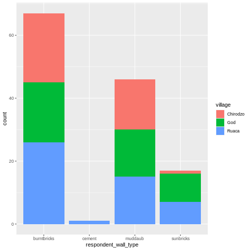
interviews_plotting %>%
  ggplot(aes(x = respondent_wall_type)) +
  geom_bar(aes(fill = village))
We can also create a caption with the chunk option
fig.cap.
```{r chunk-name, fig.cap = "I made this plot while attending an
awesome Data Carpentries workshop where I learned a ton of cool stuff!"}
Code for plot
```
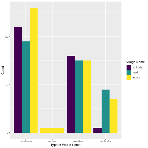
…or, ideally, something more informative.
R
interviews_plotting %>%
  ggplot(aes(x = respondent_wall_type)) +
  geom_bar(aes(fill = village), position = "dodge") +
  labs(x = "Type of Wall in Home", y = "Count", fill = "Village Name") +
  scale_fill_viridis_d() # add colour deficient friendly palette
Other output options
You can convert R Markdown to a PDF or a Word document (among
others). Click the little triangle next to the Knit
button to get a drop-down menu. Or you could put
pdf_document or word_document in the initial
header of the file.
---
title: "My Awesome Report"
author: "Emmet Brickowski"
date: ""
output: word_document
---
Note: Creating PDF documents
Creating .pdf documents may require installation of some extra
software. The R package tinytex provides some tools to help
make this process easier for R users. With tinytex
installed, run tinytex::install_tinytex() to install the
required software (you’ll only need to do this once) and then when you
Knit to pdf tinytex will automatically
detect and install any additional LaTeX packages that are needed to
produce the pdf document. Visit the tinytex website for more
information.