Working with skimage
Last updated on 2023-04-25 | Edit this page
Overview
Questions
- How can the skimage Python computer vision library be used to work with images?
Objectives
- Read and save images with imageio.
- Display images with matplotlib.
- Resize images with skimage.
- Perform simple image thresholding with NumPy array operations.
- Extract sub-images using array slicing.
We have covered much of how images are represented in computer software. In this episode we will learn some more methods for accessing and changing digital images.
First, import the packages needed for this episode
Reading, displaying, and saving images
Imageio provides intuitive functions for reading and writing (saving) images. All of the popular image formats, such as BMP, PNG, JPEG, and TIFF are supported, along with several more esoteric formats. Check the Supported Formats docs for a list of all formats. Matplotlib provides a large collection of plotting utilities.
Let us examine a simple Python program to load, display, and save an image to a different format. Here are the first few lines:
PYTHON
"""
 * Python program to open, display, and save an image.
 *
"""
# read image
chair = iio.imread(uri="data/chair.jpg")
We use the iio.imread() function to read a JPEG image
entitled chair.jpg. Imageio reads the image, converts
it from JPEG into a NumPy array, and returns the array; we save the
array in a variable named image.
Next, we will do something with the image:
Once we have the image in the program, we first call
plt.subplots() so that we will have a fresh figure with a
set of axis independent from our previous calls. Next we call
plt.imshow() in order to display the image.
Now, we will save the image in another format:
The final statement in the program,
iio.imwrite(uri="data/chair.tif", image=chair), writes the
image to a file named chair.tif in the data/
directory. The imwrite() function automatically determines
the type of the file, based on the file extension we provide. In this
case, the .tif extension causes the image to be saved as a
TIFF.
Metadata, revisited
Remember, as mentioned in the previous section, images saved with
imwrite() will not retain all metadata associated with the
original image that was loaded into Python! If the image metadata
is important to you, be sure to always keep an unchanged copy of
the original image!
Extensions do not always dictate file type
The iio.imwrite() function automatically uses the file
type we specify in the file name parameter’s extension. Note that this
is not always the case. For example, if we are editing a document in
Microsoft Word, and we save the document as paper.pdf
instead of paper.docx, the file is not saved as a
PDF document.
Named versus positional arguments
When we call functions in Python, there are two ways we can specify the necessary arguments. We can specify the arguments positionally, i.e., in the order the parameters appear in the function definition, or we can use named arguments.
For example, the iio.imwrite() function
definition specifies two parameters, the resource to save the image
to (e.g., a file name, an http address) and the image to write to disk.
So, we could save the chair image in the sample code above using
positional arguments like this:
iio.imwrite("data/chair.tif", image)
Since the function expects the first argument to be the file name,
there is no confusion about what "data/chair.jpg" means.
The same goes for the second argument.
The style we will use in this workshop is to name each argument, like this:
iio.imwrite(uri="data/chair.tif", image=image)
This style will make it easier for you to learn how to use the variety of functions we will cover in this workshop.
Resizing an image (10 min)
Add import skimage.transform and
import skimage.util to your list of imports. Using the
chair.jpg image located in the data folder, write a Python
script to read your image into a variable named chair.
Then, resize the image to 10 percent of its current size using these
lines of code:
PYTHON
new_shape = (chair.shape[0] // 10, chair.shape[1] // 10, chair.shape[2])
resized_chair = skimage.transform.resize(image=chair, output_shape=new_shape)
resized_chair = skimage.util.img_as_ubyte(resized_chair)As it is used here, the parameters to the
skimage.transform.resize() function are the image to
transform, chair, the dimensions we want the new image to
have, new_shape.
Callout
Note that the pixel values in the new image are an approximation of
the original values and should not be confused with actual, observed
data. This is because skimage interpolates the pixel values
when reducing or increasing the size of an image.
skimage.transform.resize has a number of optional
parameters that allow the user to control this interpolation. You can
find more details in the scikit-image
documentation.
Image files on disk are normally stored as whole numbers for space
efficiency, but transformations and other math operations often result
in conversion to floating point numbers. Using the
skimage.util.img_as_ubyte() method converts it back to
whole numbers before we save it back to disk. If we don’t convert it
before saving, iio.imwrite() may not recognise it as image
data.
Next, write the resized image out to a new file named
resized.jpg in your data directory. Finally, use
plt.imshow() with each of your image variables to display
both images in your notebook. Don’t forget to use
fig, ax = plt.subplots() so you don’t overwrite the first
image with the second. Images may appear the same size in jupyter, but
you can see the size difference by comparing the scales for each. You
can also see the differnce in file storage size on disk by hovering your
mouse cursor over the original and the new file in the jupyter file
browser, using ls -l in your shell, or the OS file browser
if it is configured to show file sizes.
Here is what your Python script might look like.
PYTHON
"""
* Python script to read an image, resize it, and save it
* under a different name.
"""
# read in image
chair = iio.imread(uri="data/chair.jpg")
# resize the image
new_shape = (chair.shape[0] // 10, chair.shape[1] // 10, chair.shape[2])
resized_chair = skimage.transform.resize(image=chair, output_shape=new_shape)
resized_chair = skimage.util.img_as_ubyte(resized_chair)
# write out image
iio.imwrite(uri="data/resized_chair.jpg", image=resized_chair)
# display images
fig, ax = plt.subplots()
plt.imshow(chair)
fig, ax = plt.subplots()
plt.imshow(resized_chair)The script resizes the data/chair.jpg image by a factor
of 10 in both dimensions, saves the result to the
data/resized_chair.jpg file, and displays original and
resized for comparision.
Manipulating pixels
In the Image Basics episode, we individually manipulated the colours of pixels by changing the numbers stored in the image’s NumPy array. Let’s apply the principles learned there along with some new principles to a real world example.
Suppose we are interested in this maize root cluster image. We want to be able to focus our program’s attention on the roots themselves, while ignoring the black background.
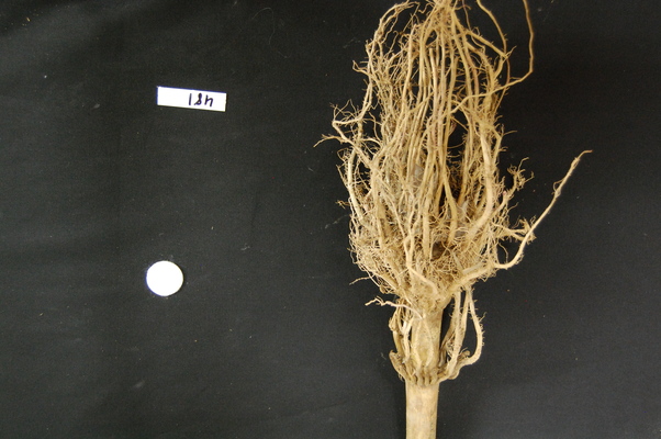
Since the image is stored as an array of numbers, we can simply look through the array for pixel colour values that are less than some threshold value. This process is called thresholding, and we will see more powerful methods to perform the thresholding task in the Thresholding episode. Here, though, we will look at a simple and elegant NumPy method for thresholding. Let us develop a program that keeps only the pixel colour values in an image that have value greater than or equal to 128. This will keep the pixels that are brighter than half of “full brightness”, i.e., pixels that do not belong to the black background.
We will start by reading the image and displaying it.
Loading images with imageio:
Read-only arrays
When loading an image with imageio, in certain
situations the image is stored in a read-only array. If you attempt to
manipulate the pixels in a read-only array, you will receive an error
message ValueError: assignment destination is read-only. In
order to make the image array writeable, we can create a copy with
image = np.array(image) before manipulating the pixel
values.
PYTHON
"""
* Python script to ignore low intensity pixels in an image.
*
"""

# read input image
maize_roots = iio.imread(uri="data/maize-root-cluster.jpg")
maize_roots = np.array(maize_roots)

# display original image
fig, ax = plt.subplots()
plt.imshow(maize_roots)
Now we can threshold the image and display the result.
PYTHON
# keep only high-intensity pixels
maize_roots[maize_roots < 128] = 0
# display modified image
fig, ax = plt.subplots()
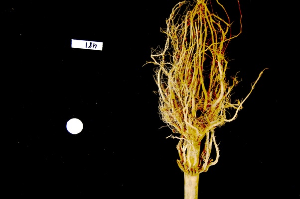
plt.imshow(maize_roots)The NumPy command to ignore all low-intensity pixels is
roots[roots < 128] = 0. Every pixel colour value in the
whole 3-dimensional array with a value less that 128 is set to zero. In
this case, the result is an image in which the extraneous background
detail has been removed.
Converting colour images to grayscale
It is often easier to work with grayscale images, which have a single
channel, instead of colour images, which have three channels. Skimage
offers the function skimage.color.rgb2gray() to achieve
this. This function adds up the three colour channels in a way that
matches human colour perception, see the
skimage documentation for details. It returns a grayscale image with
floating point values in the range from 0 to 1. We can use the function
skimage.util.img_as_ubyte() in order to convert it back to
the original data type and the data range back 0 to 255. Note that it is
often better to use image values represented by floating point values,
because using floating point numbers is numerically more stable.
Colour and color
The Carpentries generally prefers UK English spelling, which is why
we use “colour” in the explanatory text of this lesson. However,
skimage contains many modules and functions that include
the US English spelling, color. The exact spelling matters
here, e.g. you will encounter an error if you try to run
skimage.colour.rgb2gray(). To account for this, we will use
the US English spelling, color, in example Python code
throughout the lesson. You will encounter a similar approach with
“centre” and center.
PYTHON
"""
* Python script to load a color image as grayscale.
*
"""

# read input image
chair = iio.imread(uri="data/chair.jpg")

# display original image
fig, ax = plt.subplots()
plt.imshow(chair)

# convert to grayscale and display
gray_chair = skimage.color.rgb2gray(chair)
fig, ax = plt.subplots()
plt.imshow(gray_chair, cmap="gray")
We can also load colour images as grayscale directly by passing the
argument mode="L" to iio.imread().
PYTHON
"""
* Python script to load a color image as grayscale.
*
"""

# read input image, based on filename parameter
gray_chair = iio.imread(uri="data/chair.jpg", mode="L")

# display grayscale image
fig, ax = plt.subplots()
plt.imshow(gray_chair, cmap="gray")
The first argument to iio.imread() is the filename of
the image. The second argument mode="L" determines the type
and range of the pixel values in the image (e.g., an 8-bit pixel has a
range of 0-255). This argument is forwarded to the pillow
backend, a Python imaging library for which mode “L” means 8-bit pixels
and single-channel (i.e., grayscale). The backend used by
iio.imread() may be specified as an optional argument: to
use pillow, you would pass plugin="pillow". If
the backend is not specified explicitly, iio.imread()
determines the backend to use based on the image type.
Loading images with imageio:
Pixel type and depth
When loading an image with mode="L", the pixel values
are stored as 8-bit integer numbers that can take values in the range
0-255. However, pixel values may also be stored with other types and
ranges. For example, some skimage functions return the
pixel values as floating point numbers in the range 0-1. The type and
range of the pixel values are important for the colorscale when
plotting, and for masking and thresholding images as we will see later
in the lesson. If you are unsure about the type of the pixel values, you
can inspect it with print(image.dtype). For the example
above, you should find that it is dtype('uint8') indicating
8-bit integer numbers.
Keeping only low intensity pixels (10 min)
A little earlier, we showed how we could use Python and skimage to turn on only the high intensity pixels from an image, while turning all the low intensity pixels off. Now, you can practice doing the opposite - keeping all the low intensity pixels while changing the high intensity ones.
The file data/sudoku.png is an RGB image of a sudoku
puzzle:
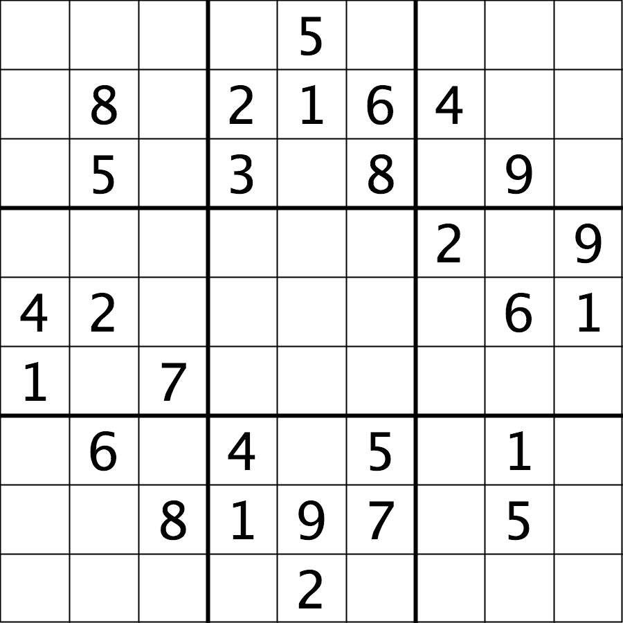
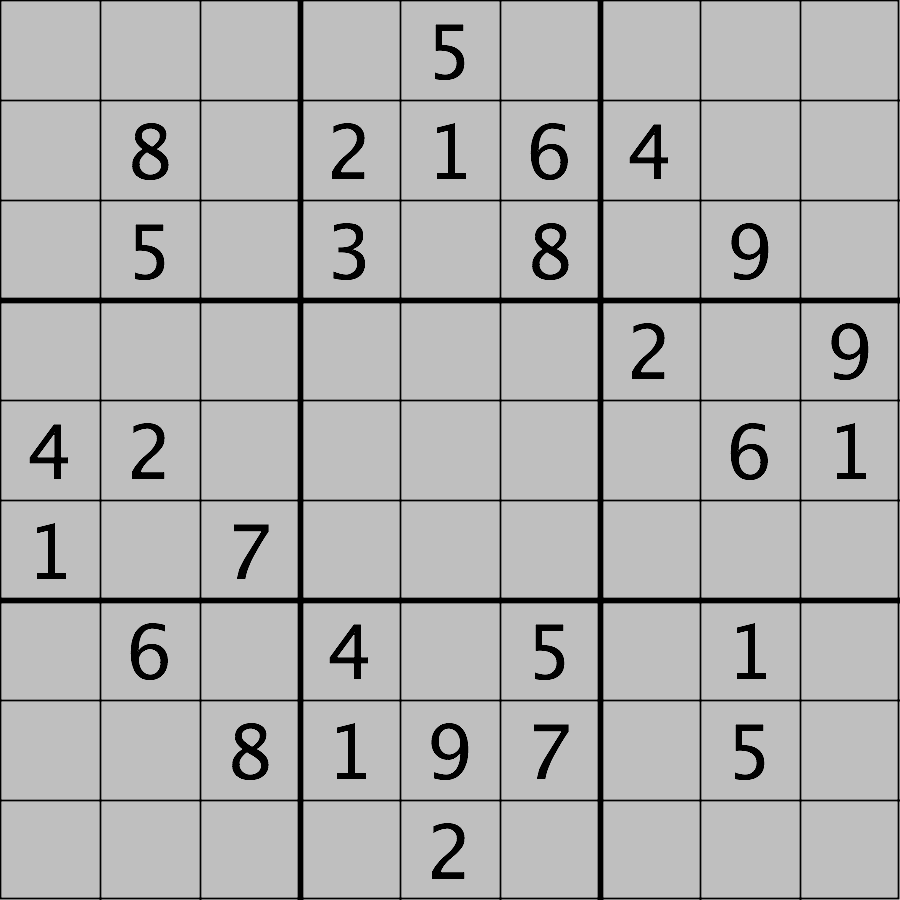
Your task is to turn all of the bright pixels in the image to a light gray colour. In other words, mask the bright pixels that have a pixel value greater than, say, 192 and set their value to 192 (the value 192 is chosen here because it corresponds to 75% of the range 0-255 of an 8-bit pixel). The results should look like this:
Hint: this is an instance where it is helpful to load the image in grayscale format.
First, load the image file data/sudoku.png as a
grayscale image. Remember that we use
image = np.array(image) to create a copy of the image array
because imageio returns a non-writeable image.
Then change all bright pixel values greater than 192 to 192:
Finally, display the modified image. Note that we have to specify
vmin=0 and vmax=255 as the range of the
colorscale because it would otherwise automatically adjust to the new
range 0-192.
Plotting single channel images (cmap, vmin, vmax)
Compared to a colour image, a grayscale image contains only a single
intensity value per pixel. When we plot such an image with
plt.imshow, matplotlib uses a colour map, to assign each
intensity value a colour. The default colour map is called “viridis” and
maps low values to purple and high values to yellow. We can instruct
matplotlib to map low values to black and high values to white instead,
by calling plt.imshow with cmap="gray". The
documentation contains an overview of pre-defined colour maps.
Furthermore, matplotlib determines the minimum and maximum values of
the colour map dynamically from the image, by default. That means that
in an image where the minimum is 64 and the maximum is 192, those values
will be mapped to black and white respectively (and not dark gray and
light gray as you might expect). If there are defined minimum and
maximum vales, you can specify them via vmin and
vmax to get the desired output.
If you forget about this, it can lead to unexpected results. Try
removing the vmax parameter from the sudoku challenge
solution and see what happens.
Access via slicing
As noted in the previous lesson skimage images are stored as NumPy arrays, so we can use array slicing to select rectangular areas of an image. Then, we can save the selection as a new image, change the pixels in the image, and so on. It is important to remember that coordinates are specified in (ry, cx) order and that colour values are specified in (r, g, b) order when doing these manipulations.
Consider this image of a whiteboard, and suppose that we want to create a sub-image with just the portion that says “odd + even = odd,” along with the red box that is drawn around the words.
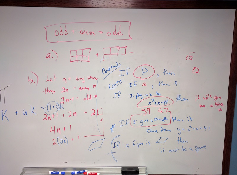
Using the same display technique we have used throughout this course, we can determine the coordinates of the corners of the area we wish to extract by hovering the mouse near the points of interest and noting the coordinates. If we do that, we might settle on a rectangular area with an upper-left coordinate of (135, 60) and a lower-right coordinate of (480, 150), as shown in this version of the whiteboard picture:
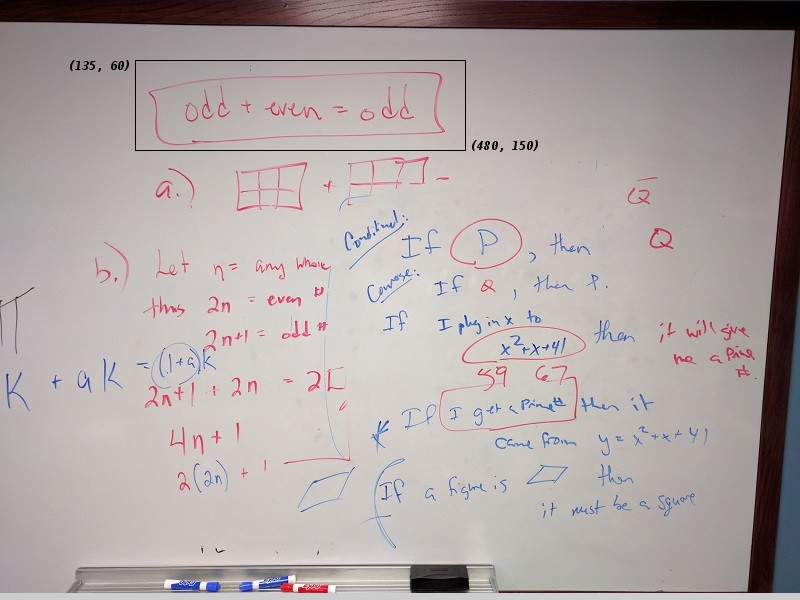
Note that the coordinates in the preceding image are specified in
(cx, ry) order. Now if our entire whiteboard image is stored as
an skimage image named image, we can create a new image of
the selected region with a statement like this:
clip = image[60:151, 135:481, :]
Our array slicing specifies the range of y-coordinates or rows first,
60:151, and then the range of x-coordinates or columns,
135:481. Note we go one beyond the maximum value in each
dimension, so that the entire desired area is selected. The third part
of the slice, :, indicates that we want all three colour
channels in our new image.
A script to create the subimage would start by loading the image:
PYTHON
"""
 * Python script demonstrating image modification and creation via
 * NumPy array slicing.
"""

# load and display original image
board = iio.imread(uri="data/board.jpg")
board = np.array(board)
fig, ax = plt.subplots()
plt.imshow(board)
Then we use array slicing to create a new image with our selected area and then display the new image.
PYTHON
# extract, display, and save sub-image
clipped_board = board[60:151, 135:481, :]
fig, ax = plt.subplots()
plt.imshow(clipped_board)
iio.imwrite(uri="data/clipped_board.tif", image=clipped_board)
We can also change the values in an image, as shown next.
PYTHON
# replace clipped area with sampled color
color = board[330, 90]
board[60:151, 135:481] = color
fig, ax = plt.subplots()
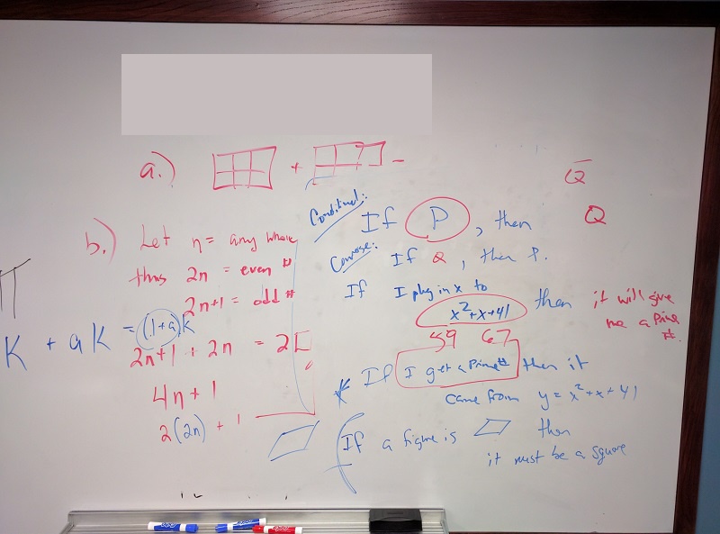
plt.imshow(board)First, we sample a single pixel’s colour at a particular location of
the image, saving it in a variable named color, which
creates a 1 × 1 × 3 NumPy array with the blue, green, and red colour
values for the pixel located at (ry = 330, cx = 90). Then, with
the img[60:151, 135:481] = color command, we modify the
image in the specified area. From a NumPy perspective, this changes all
the pixel values within that range to array saved in the
color variable. In this case, the command “erases” that
area of the whiteboard, replacing the words with a beige colour, as
shown in the final image produced by the program:
Practicing with slices (10 min - optional, not included in timing)
Using the techniques you just learned, write a script that creates, displays, and saves a sub-image containing only the plant and its roots from “data/maize-root-cluster.jpg”
Here is the completed Python program to select only the plant and roots in the image.
PYTHON
"""
 * Python script to extract a sub-image containing only the plant and
 * roots in an existing image.
"""

# load and display original image
maize_roots = iio.imread(uri="data/maize-root-cluster.jpg")
fig, ax = plt.subplots()
plt.imshow(maize_roots)

# extract, display, and save sub-image
# WRITE YOUR CODE TO SELECT THE SUBIMAGE NAME clip HERE:
clipped_maize = maize_roots[0:400, 275:550, :]
fig, ax = plt.subplots()
plt.imshow(clipped_maize)


# WRITE YOUR CODE TO SAVE clip HERE
iio.imwrite(uri="data/clipped_maize.jpg", image=clipped_maize)
Key Points
- Images are read from disk with the
iio.imread()function. - We create a window that automatically scales the displayed image
with matplotlib and calling
show()on the global figure object. - Colour images can be transformed to grayscale using
skimage.color.rgb2gray()or, in many cases, be read as grayscale directly by passing the argumentmode="L"toiio.imread(). - We can resize images with the
skimage.transform.resize()function. - NumPy array commands, such as
image[image < 128] = 0, can be used to manipulate the pixels of an image. - Array slicing can be used to extract sub-images or modify areas of
images, e.g.,
clip = image[60:150, 135:480, :]. - Metadata is not retained when images are loaded as skimage images.